Hate Speech Detection using Deep Learning (original) (raw)

Last Updated : 23 Jul, 2025

There must be times when you have come across some social media post whose main aim is to spread hate and controversies or use abusive language on social media platforms. As the post consists of textual information to filter out such Hate Speeches NLP comes in handy. This is one of the main applications of NLP which is known as Sentence Classification tasks.

In this article we’ll walk through a stepwise implementation of building an NLP-based sequence classification model to classify tweets as Hate Speech, Offensive Language or Neutral .

**Step 1: Importing Required Libraries

Before we begin let’s import the necessary libraries for data processing, model building and visualization.

Python `

%%capture import numpy as np import pandas as pd import matplotlib.pyplot as plt import seaborn as sb from sklearn.model_selection import train_test_split

import nltk import string import warnings from nltk.corpus import stopwords from nltk.stem import WordNetLemmatizer from wordcloud import WordCloud

import tensorflow as tf from tensorflow import keras from keras import layers from tensorflow.keras.preprocessing.text import Tokenizer from tensorflow.keras.preprocessing.sequence import pad_sequences

nltk.download('stopwords') nltk.download('omw-1.4') nltk.download('wordnet') warnings.filterwarnings('ignore')

`

**Step 2: Loading the Dataset

We’ll use the Hate Speech Dataset which contains labeled tweets classified into three categories:

• **0 - Hate Speech : Content explicitly targeting individuals or groups with harmful intent.
• **1 - Offensive Language : Content containing offensive language but not necessarily hate speech.
• **2 - Neither : Neutral content without any offensive or hateful intent.

The dataset consists of 19,826 rows and 2 columns : tweet (textual content) and class (label). Let’s load the dataset and explore its structure. You can download the dataset from here.

Python `

df = pd.read_csv('hate_speech.csv') df.head()

`

**Output:

First Five rows of the dataset

To check how many such tweets data we have let's print the shape of the data frame.

Python `

df.shape

`

**Output:

(24783, 2)

Although there are only two columns in this dataset let's check the info about their columns.

Python `

df.info()

`

**Output:

Info about the dataset

The shape of the data frame and the number of non-null values are the same hence we can say that there are no null values in the dataset.

Python `

plt.pie(df['class'].value_counts().values, labels = df['class'].value_counts().index, autopct='%1.1f%%') plt.show()

`

**Output:

Here the three labels are as follows:

• 0 - Hate Speech
• 1 - Offensive Language
• 2 - Neither

**Step 3: Balancing the Dataset

The dataset is imbalanced so we balance it using a combination of upsampling and downsampling.

Python `

class_0 = df[df['class'] == 0] # Hate Speech class_1 = df[df['class'] == 1].sample(n=3500, random_state=42) # Offensive Language class_2 = df[df['class'] == 2] # Neutral

balanced_df = pd.concat([class_0, class_0, class_0, class_1, class_2], axis=0)

Visualize the balanced distribution

plt.pie(balanced_df['class'].value_counts().values, labels=balanced_df['class'].value_counts().index, autopct='%1.1f%%') plt.title("Balanced Class Distribution") plt.show()

`

**Output:

Step 4: Text Preprocessing

Textual data is highly unstructured and need attention on many aspects like:

• Stopwords Removal
• Punctuations Removal
• Stemming or Lemmatization

Although removing data means loss of information but we need to do this to make the data perfect to feed into a machine learning model.

Python `

df['tweet'] = df['tweet'].str.lower()

punctuations_list = string.punctuation def remove_punctuations(text): temp = str.maketrans('', '', punctuations_list) return text.translate(temp)

df['tweet']= df['tweet'].apply(lambda x: remove_punctuations(x)) df.head()

`

**Output:

Dataset after removal of punctuation's

The below function is a helper function that will help us to remove the stop words and Lemmatize the important words.

Python `

def preprocess_text(text): stop_words = set(stopwords.words('english')) lemmatizer = WordNetLemmatizer() words = [lemmatizer.lemmatize(word) for word in text.split() if word not in stop_words] return " ".join(words)

balanced_df['tweet'] = balanced_df['tweet'].apply(preprocess_text)

`

Word cloud is a text visualization tool that help's us to get insights into the most frequent words present in the corpus of the data.

Python `

def plot_word_cloud(data, typ): corpus = " ".join(data['tweet']) wc = WordCloud(max_words=100, width=800, height=400, collocations=False).generate(corpus) plt.figure(figsize=(10, 5)) plt.imshow(wc, interpolation='bilinear') plt.axis('off') plt.title(f"Word Cloud for {typ} Class", fontsize=15) plt.show()

plot_word_cloud(balanced_df[balanced_df['class'] == 2], typ="Neutral")

`

**Output:

**Step 5: Tokenization and Padding

In this step we convert text data into numerical sequences and pad them to a fixed length

Python `

features = balanced_df['tweet'] target = balanced_df['class'] X_train, X_val, Y_train, Y_val = train_test_split(features, target, test_size=0.2, random_state=42)

One-hot encode the labels

Y_train = pd.get_dummies(Y_train) Y_val = pd.get_dummies(Y_val)

Tokenization

max_words = 5000 max_len = 100 tokenizer = Tokenizer(num_words=max_words, lower=True, split=' ') tokenizer.fit_on_texts(X_train)

Convert text to sequences

X_train_seq = tokenizer.texts_to_sequences(X_train) X_val_seq = tokenizer.texts_to_sequences(X_val)

Pad sequences

X_train_padded = pad_sequences(X_train_seq, maxlen=max_len, padding='post', truncating='post') X_val_padded = pad_sequences(X_val_seq, maxlen=max_len, padding='post', truncating='post')

`

**Step 6: Build the Model

We will implement a Sequential model like LSTM which will contain the following parts:

• **Embedding Layers to learn a featured vector representations of the input vectors.
• **Bidirectional LSTM layer to identify useful patterns in the sequence.
• We have included **BatchNormalization layers to enable stable and fast training and a **Dropout layer before the final layer to avoid any possibility of overfitting.

The final layer is the output layer which outputs soft probabilities for the three classes.

While compiling a model we provide these three essential parameters:

• **optimizer - This is the method that helps to optimize the cost function by using gradient descent.
• **loss - The loss function by which we monitor whether the model is improving with training or not.
• **metrics - This helps to evaluate the model by predicting the training and the validation data. Python `

from tensorflow import keras from tensorflow.keras import layers

max_words = 10000 max_len = 100

model = keras.models.Sequential([ layers.Embedding(input_dim=max_words, output_dim=32, input_length=max_len), layers.Bidirectional(layers.LSTM(16)), layers.Dense(512, activation='relu', kernel_regularizer='l1'), layers.BatchNormalization(), layers.Dropout(0.3), layers.Dense(3, activation='softmax')
])

model.build(input_shape=(None, max_len))

model.compile(loss='categorical_crossentropy', optimizer='adam', metrics=['accuracy'])

model.summary()

`

**Output:

Model Training

**Step 7: Training the Model

Train the model using callbacks like EarlyStopping and ReduceLROnPlateau.

Python `

from keras.callbacks import EarlyStopping, ReduceLROnPlateau

es = EarlyStopping(patience=3, monitor='val_accuracy', restore_best_weights=True) lr = ReduceLROnPlateau(patience=2, monitor='val_loss', factor=0.5, verbose=0)

`

Let's now train the model:

Python `

history = model.fit(X_train_padded, Y_train, validation_data=(X_val_padded, Y_val), epochs=50, batch_size=32, callbacks=[es, lr])

`

**Output:

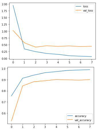
**Step 8: Evaluating the Model

Visualize the training progress and evaluate the model’s performance.

Python `

history_df = pd.DataFrame(history.history)

history_df[['loss', 'val_loss']].plot(title="Loss")

history_df[['accuracy', 'val_accuracy']].plot(title="Accuracy") plt.show()

`

**Output:

**Test Accuracy

Python `

test_loss, test_acc = model.evaluate(X_val_padded, Y_val) print(f"Validation Accuracy: {test_acc:.2f}")

`

**Output:

75/75 ━━━━━━━━━━━━━━━━━━━━ 1s 12ms/step - accuracy: 0.9182 - loss: 0.446
Validation Accuracy: 0.91

The trained model achieves 90% accuracy on the validation set, demonstrating the effectiveness of deep learning techniques like LSTM for hate speech detection. While the model shows some overfitting, regularization techniques can be applied to improve generalization.

**Get the Complete Notebook

**Notebook: **click here.