Latent Space in Deep Learning (original) (raw)

Last Updated : 14 Apr, 2026

In deep learning, latent space refers to an abstract, lower-dimensional representation of data that captures its essential features and underlying patterns. It is generated by neural networks and is termed “latent” because it encodes hidden characteristics that are not directly observable in the original input.

• Represents data in a compact and meaningful form
• Captures important patterns while removing unnecessary details
• Places similar data points closer together in the representation space
• Helps models process and understand complex data more effectively

Need of Latent Space Matters in Deep Learning

1. **Dimensionality Reduction: Latent space enables the reduction of the input data’s dimensionality while retaining essential features. This compression makes it easier to handle and process complex data.
2. **Feature Learning: By encoding data into a latent space, neural networks can learn meaningful features and patterns that are not immediately apparent in the raw data.
3. **Generative Modeling: In generative models, latent space is used to sample new data points. This capability is important for tasks such as image synthesis and text generation.

Latent Space in Different Types of Neural Networks

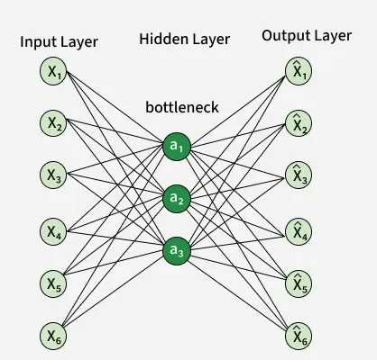
**1. Autoencoders

Autoencoder

Autoencoders are neural networks designed to learn efficient encodings of data. They consist of two main components:

• **Encoder: Maps the input data to the latent space.
• **Decoder: Reconstructs the data from the latent space representation.

The latent space in autoencoders is important because it contains a compressed version of the input data. By minimizing the reconstruction error, autoencoders learn to represent the data in a lower-dimensional space while preserving its essential characteristics.

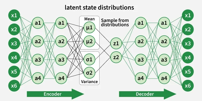
**2. Variational Autoencoders (VAEs)

VAE

VAEs extend the concept of autoencoders by introducing probabilistic elements into the latent space. Instead of learning a deterministic mapping, VAEs learn a distribution over the latent space. This allows them to generate new, diverse samples by sampling from this learned distribution.

Key components of VAEs include:

• **Encoder: Outputs parameters of a probability distribution (mean and variance) rather than a fixed latent vector.
• **Decoder: Reconstructs the data from samples drawn from the latent distribution.

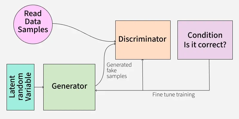
**3. Generative Adversarial Networks (GANs)

GANs use latent space to generate new data samples through a two-network setup:

GAN

• **Generator: Takes a random vector from the latent space and generates data samples.
• **Discriminator: Distinguishes between real data samples and those generated by the generator.

The latent space in GANs represents a range of possible data samples and the generator learns to map points in this space to realistic data.

**4. Recurrent Neural Networks (RNNs) and Long Short-Term Memory Networks (LSTMs)

In sequence modeling tasks, RNNs and LSTMs use latent space to capture the temporal dependencies and hidden states of the data. The latent space in these models helps in summarizing past information and predicting future sequences.

RNN

• **Hidden States: Hidden states store information from previous time steps and help capture temporal dependencies.
• **Cell States (LSTMs): Capture long-term dependencies and are part of the latent space in LSTMs.

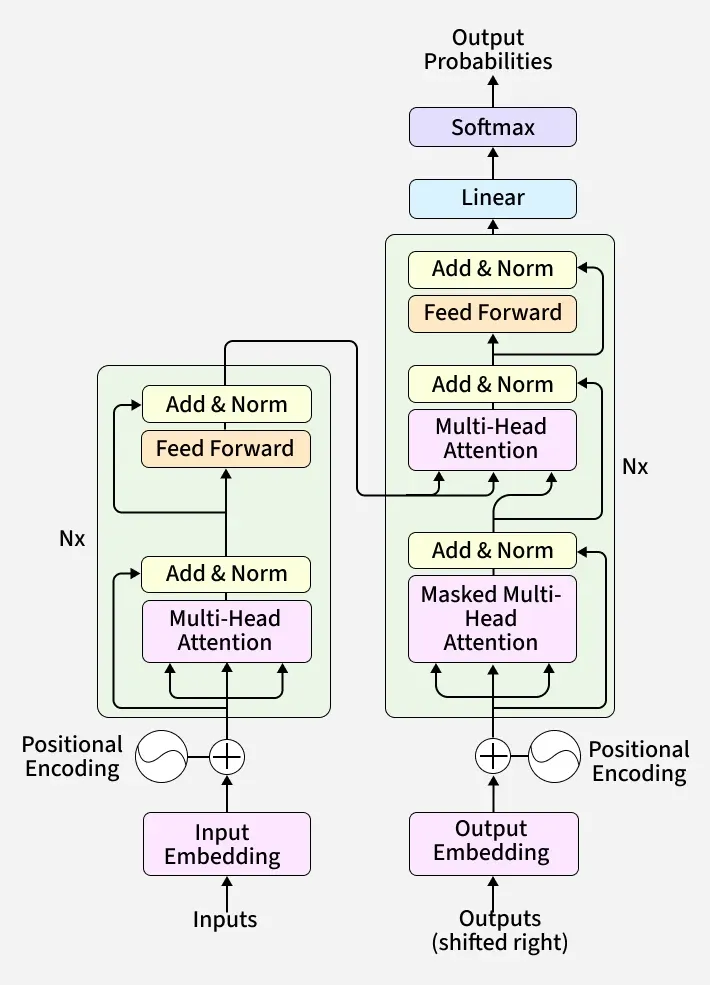
**5. Transformers

Transformers, used extensively in natural language processing, also utilize latent space. The model represents each input token in a high-dimensional space and processes it through attention mechanisms.

Transformer

• **Attention Mechanism: Allows the model to focus on different parts of the input data, effectively working with latent representations to understand context and relationships between tokens.

Visualizing Latent Space

Visualizing latent space can provide insights into how a model represents data. Techniques such ast-SNE (t-Distributed Stochastic Neighbor Embedding) and PCA (Principal Component Analysis) are often used to project high-dimensional latent spaces into 2D or 3D for visualization.

• **Principal Component Analysis (PCA): Captures the directions of maximum variance in data, helpful for understanding principal trends.
• **t-Distributed Stochastic Neighbor Embedding (t-SNE): Focuses on preserving local relationships, useful for visualizing clusters and neighborhood structures.

For example, an autoencoder trained on the MNIST dataset learns a 32-dimensional latent space encoding digit images. Applying PCA or t-SNE on this space reveals well-separated clusters corresponding to digit classes, illustrating the model's effective feature extraction.

• Uniform Manifold Approximation and Projection (**UMAP**)**: Balances global and local structure preservation, scalable for larger datasets.

Visualizing Latent Space using PCA

In this section, we are going to visualize latent space using PCA by following these steps:

1. **Data Preprocessing: We normalize the MNIST dataset and flatten the images for the autoencoder.
2. **Autoencoder Architecture: The autoencoder consists of an encoder that compresses the data into a latent space and a decoder that reconstructs the original data from the latent space.
3. **Training: We train the autoencoder on the MNIST dataset, which helps the model learn meaningful representations in the latent space.
4. **Dimensionality Reduction: We use PCA to reduce the latent space dimensions to 2D for visualization. Alternatively, you can use t-SNE for potentially better visual separation.
5. **Plotting: We use Matplotlib to create scatter plots of the latent space representations, providing a visual understanding of how the model organizes the data.

Step 1: Import Libraries and Load Data

Load the MNIST dataset and preprocess by normalizing and flattening images for input to the neural network.

Python `

import numpy as np import matplotlib.pyplot as plt from sklearn.decomposition import PCA from tensorflow.keras.layers import Input, Dense from tensorflow.keras.models import Model from tensorflow.keras.datasets import mnist

(x_train, _), (x_test, _) = mnist.load_data()

x_train = x_train.astype('float32') / 255.0 x_test = x_test.astype('float32') / 255.0

x_train = x_train.reshape((x_train.shape[0], 2828)) x_test = x_test.reshape((x_test.shape[0], 2828))

`

Step 2: Define Autoencoder Architecture

Define a simple autoencoder with one hidden layer that compresses data to a 32-dimensional latent space and reconstructs it back.

Python `

input_dim = x_train.shape[1]
encoding_dim = 32

input_layer = Input(shape=(input_dim,)) encoded = Dense(encoding_dim, activation='relu')(input_layer)

decoded = Dense(input_dim, activation='sigmoid')(encoded)

autoencoder = Model(input_layer, decoded)

encoder = Model(input_layer, encoded)

`

Step 3: Compile and Train the Autoencoder

Compile the model with Adam optimizer and binary cross-entropy loss. Train the autoencoder to minimize reconstruction error.

Python `

autoencoder.compile(optimizer='adam', loss='binary_crossentropy')

Train for 50 epochs with batch size 256

autoencoder.fit(x_train, x_train, epochs=50, batch_size=256, shuffle=True, validation_data=(x_test, x_test))

`

**Output:

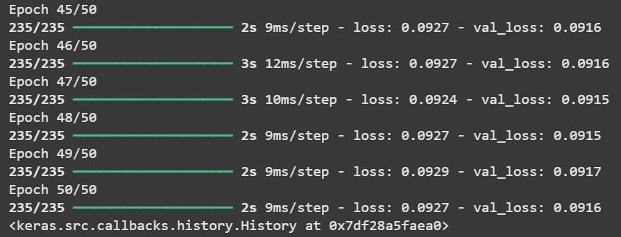
Training

Use the trained encoder to obtain 32-dimensional latent representations of the training and testing data.

Python `

latent_space_train = encoder.predict(x_train) latent_space_test = encoder.predict(x_test)

`

**Output:

1875/1875 ━━━━━━━━━━━━━━━━━━━━ 2s 977us/step
313/313 ━━━━━━━━━━━━━━━━━━━━ 0s 1ms/step

Step 5: Apply PCA for Dimensionality Reduction

Reduce the 32-dimensional latent space to 2D using PCA to enable visualization.

Python `

pca = PCA(n_components=2)

latent_space_train_pca = pca.fit_transform(latent_space_train) latent_space_test_pca = pca.transform(latent_space_test)

`

Step 6: Visualize the Latent Space

Plot the 2D PCA projection of latent space to visualize how data points cluster or spread in the learned space.

Python `

plt.figure(figsize=(10, 8)) plt.scatter(latent_space_train_pca[:, 0], latent_space_train_pca[:, 1], s=1, label='Training data') plt.scatter(latent_space_test_pca[:, 0], latent_space_test_pca[:, 1], s=1, label='Testing data', alpha=0.5) plt.xlabel('Principal Component 1') plt.ylabel('Principal Component 2') plt.title('Latent Space Visualization using PCA') plt.legend() plt.show()

`

**Output:

PCA

Visualizing Latent Space using t-SNE

To visualize the latent space using t-SNE (t-Distributed Stochastic Neighbor Embedding), follow the steps below:

1. **Data Preprocessing: The MNIST dataset is normalized and reshaped. Each image is converted from 28x28 to a 784-dimensional vector.
2. **Autoencoder Model: We create an autoencoder with a simple architecture for this example. The encoder compresses the data into the latent space and the decoder reconstructs the original data.
3. **Training: The autoencoder is trained to minimize the reconstruction loss, learning to map the data into the latent space effectively.
4. **Latent Space Representation: After training, we extract the latent space representations using the encoder.
5. **Dimensionality Reduction with t-SNE: t-SNE is applied to reduce the latent space dimensions to 2D. This technique helps in visualizing how data points are distributed in the latent space and can reveal clusters and structures that are not apparent in higher dimensions.
6. **Plotting: We use Matplotlib to create scatter plots of the t-SNE reduced latent space. Different colors or markers can be used to distinguish between training and testing data.

Here’s the step-by-step implementation

**Step 1: Apply t-SNE on Latent Space

We first import the TSNE class from sklearn.manifold and configure it with the required parameters.

• n_components=2: Reduces data to 2 dimensions for easy visualization.
• random_state=42: Ensures reproducible results.
• perplexity=30: Balances local and global aspects of the data.
• n_iter=1000: Defines the number of optimization iterations. Python `

from sklearn.manifold import TSNE tsne = TSNE(n_components=2, random_state=42, perplexity=30, n_iter=1000)

`

Step 2: Transforming Datapoints

Next, we apply fit_transform() to both training and testing latent space representations.

• latent_space_train[:5000]: Only the first 5000 samples are used for faster computation since t-SNE is slow on large datasets.
• fit_transform(): Fits the model and reduces data to 2D.
• Separate transformations are applied to training and test data. Python `

latent_space_train_tsne = tsne.fit_transform(latent_space_train[:5000]) latent_space_test_tsne = tsne.fit_transform(latent_space_test[:1000])

`

Step 3: Visualize the latent space using t-SNE

Plots scatter points for the test data with similar coordinates.

Python `

plt.figure(figsize=(10, 8)) plt.scatter(latent_space_train_tsne[:, 0], latent_space_train_tsne[:, 1], s=1, label='Training data') plt.scatter(latent_space_test_tsne[:, 0], latent_space_test_tsne[:, 1], s=1, label='Testing data', alpha=0.5) plt.xlabel('t-SNE Dimension 1') plt.ylabel('t-SNE Dimension 2') plt.title('Latent Space Visualization using t-SNE') plt.legend() plt.show()

`

**Output:

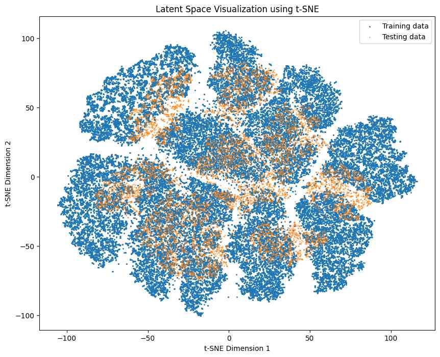
t-SNE

Visualizing Latent Space using UMAP

To visualize latent space using UMAP, you can follow these essential steps:

**1. Data Preprocessing:

• Normalize the MNIST dataset’s pixel values to the range.
• Flatten each 28x28 image into a 784-dimensional vector suitable for input into the autoencoder.

**2. Autoencoder Model:

• Build a simple autoencoder where the encoder compresses the input into a lower-dimensional latent space (e.g., 32 dimensions).
• The decoder reconstructs the input from this compact latent representation.

**3. Training: Train the autoencoder by minimizing reconstruction loss to effectively learn meaningful latent space encodings.

**4. Latent Space Representation: Use the trained encoder to extract latent representations for both training and testing data.

**5. Dimensionality Reduction with UMAP:

• Apply UMAP on the latent space vectors to reduce their dimensionality to 2D.
• UMAP preserves both local and global data structure better and scales more efficiently for larger datasets.

**6. Plotting:

• Use Matplotlib to plot the 2D UMAP embeddings as a scatter plot.
• Differentiate training and testing data points with distinct colors or markers for clear visualization.

Here’s the step-by-step implementation.

Step 1: Install UMAP

Python `

pip install umap-learn

`

Step 2: Import UMAP with other libraries

Python `

import numpy as np import matplotlib.pyplot as plt import umap from tensorflow.keras.layers import Input, Dense from tensorflow.keras.models import Model from tensorflow.keras.datasets import mnist

`

Step 3: Load and preprocess the MNIST dataset

Python `

(x_train, _), (x_test, _) = mnist.load_data() x_train = x_train.astype('float32') / 255.0 x_test = x_test.astype('float32') / 255.0 x_train = x_train.reshape((x_train.shape[0], 2828)) x_test = x_test.reshape((x_test.shape[0], 2828))

`

Step 4: Define and train the autoencoder

Python `

input_dim = x_train.shape[1] encoding_dim = 32

input_layer = Input(shape=(input_dim,)) encoded = Dense(encoding_dim, activation='relu')(input_layer) decoded = Dense(input_dim, activation='sigmoid')(encoded)

autoencoder = Model(input_layer, decoded) encoder = Model(input_layer, encoded)

autoencoder.compile(optimizer='adam', loss='binary_crossentropy') autoencoder.fit(x_train, x_train, epochs=50, batch_size=256, shuffle=True, validation_data=(x_test, x_test))

`

Step 5: Obtain latent space representations

Python `

latent_space_train = encoder.predict(x_train) latent_space_test = encoder.predict(x_test)

`

Step 6: Apply UMAP to reduce latent space dimensions to 2

Python `

reducer = umap.UMAP(n_components=2, random_state=42) latent_space_train_umap = reducer.fit_transform(latent_space_train) latent_space_test_umap = reducer.transform(latent_space_test)

`

Step 7: Visualize the 2D UMAP projections

Python `

plt.figure(figsize=(10, 8)) plt.scatter(latent_space_train_umap[:, 0], latent_space_train_umap[:, 1], s=1, label='Training data') plt.scatter(latent_space_test_umap[:, 0], latent_space_test_umap[:, 1], s=1, label='Testing data', alpha=0.5) plt.xlabel('UMAP Dimension 1') plt.ylabel('UMAP Dimension 2') plt.title('Latent Space Visualization using UMAP') plt.legend() plt.show()

`

Output:

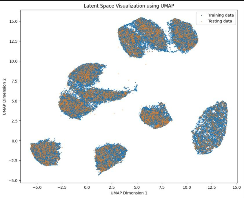
UMAP

Applications

1. **Data Compression: Latent space representations can be used for compressing data, making storage and transmission more efficient.
2. **Anomaly Detection: By analyzing the latent space, models can identify anomalies or outliers that deviate significantly from the learned distribution.
3. **Data Generation: Latent space allows for the generation of new data samples, which is valuable in creative fields such as art, music and synthetic data creation.
4. **Transfer Learning: Latent space representations learned from one domain can be transferred to other domains, facilitating knowledge transfer and improving model performance on new tasks.