Automated Music Genre Classification using Librosa and XGBOOST (original) (raw)
Last Updated : 23 Jul, 2025
Music genre classification is a critical task in the field of music information retrieval, which aims to categorize music tracks into predefined genres based on their audio features. This process is essential for organizing large music libraries, enhancing music recommendation systems, and providing valuable insights into musical trends. In this article, we will explore how to implement an automated music genre classification system using the Librosa library for feature extraction and the XGBoost algorithm for classification.
Table of Content
- Understanding Music Genre Classification
- Why Librosa for Audio Feature Extraction?
- Key Features for Music Classification
- Setting up the Dataset for Genre Classification
- Building the Music Genre Classification Model
- Challenges and Future Directions
**Understanding Music Genre Classification
**Music genre classification involves analyzing audio signals to identify the genre of a given music track. This task can be approached using various machine learning and deep learning techniques. Traditional machine learning algorithms like Support Vector Machines (SVM), k-nearest neighbors (KNN), and decision trees have been used in the past.
However, recent advancements have shown that deep learning models, particularly Convolutional Neural Networks (CNNs), often outperform traditional methods due to their ability to capture complex patterns in audio data
Librosa is a Python library that is used to extract audio features from audio files. Just like for processing images, we have Image Processing libraries, similarly to extract features from audio files and convert to vectors we use this powerful library. **Librosa provides tools for extracting various audio features such as Mel-frequency cepstral coefficients (MFCCs), chroma features, spectral contrast, and more. These features are crucial for understanding the characteristics of music tracks . Librosa is used in many cases:
- Classification: To classify to which category the music belongs.
- Speech Recognition: to identify a person's speech based on tone, pitch, frequency etc.
Key Features for Music Classification
There are different features for music classification:
- **Chroma Features: These features are basically used to capture energy or intensity of the sound. This feature is used for analysis of harmonic contents.
- **Spectral Features: This feature basically focuses on the frequency of the sound. In this basically weighted mean and range of frequencies are calculated. It includes Spectral Centroid, spectral bandwidth etc.
- **Mel-Frequency Cepstral Coefficient: These are coefficients that are calculated using Fourier transformation. This feature focuses on how humans listen to the sound. This feature basically focuses on style, tone, texture of the songs.
- **Tempo: This feature is responsible for calculating the speed of the music or in simple terms measures the number of beats per minute.
- **Tonnetz: This feature is used to capture the mood or the harmony of the music.
- **Harmonic-Percussive Source Separation (HPSS): As the name suggests this is used to separate the harmony and the beat/percussion of the audio.
- Zero Crossing Rate: This feature is used to represent the noise on number line. It basically captures the rate at which the audio changes its path.
- Root Mean S**quare En****ergy: This is used to measure the loudness of the sound.
Setting up the Dataset for Genre Classification
For this project, we will use the GTZAN Genre Classification dataset, which is widely used in academic research for music genre classification tasks. The dataset consists of 1,000 audio tracks, each 30 seconds long, categorized into 10 genres: Blues, Classical, Country, Disco, Hip-hop, Jazz, Metal, Pop, Reggae, and Rock.
The audio files are in.wav format. There are 100 files in each folder. Now we have all the contents present in zip folder which is accessible from the link. We have basically extracted them from the zip file present in the Google Drive and stored them in a directory named GTZAN/music. Inside the music folder, different genres are present.
You can get the data the zip file link:
https://drive.google.com/file/d/1MVYIGyienvBkfK9t5LP9GhobgXrTneqT/view?usp=drive\_link
Python `
import zipfile import os
Assuming the uploaded zip file is present in the drive
zip_file_path = '/content/drive/MyDrive/music.zip'
Unzip the file
with zipfile.ZipFile(zip_file_path, 'r') as zip_ref: zip_ref.extractall('/content/GTZAN')
Specify the directory containing genre folders
data_dir = "/content/GTZAN/music" # dataset path
Get the list of genre folder names
genres = [f for f in os.listdir(data_dir) if os.path.isdir(os.path.join(data_dir, f))]
Print the genres to check
print("Genres found:", genres)
`
**Output:
Genres found: ['jazz', 'classical', 'pop', 'metal', 'blues', 'rock', 'disco', 'hiphop', 'reggae', 'country']
**Building the Music Genre Classification Model
To extract features from the audio files, we need to install the librosa library. For installation use the pip command.
pip install librosa
After installing and loading the dataset, we have will now extract features like MFCC, Chroma features, Spectrum features, Zero Crossing Rates, Tonnetz and Root Mean square Energy.
- These features are concatenated and are further appended to list named 'X'. The genre names are added to variable 'y' which is basically our label.
- The try-except block is used to handle errors if Librosa cannot process the file.
- Then these features are normalized using StandardScaler.
- The labels are converted to numeric labels using Label Encoder.
- The data has been divided in the ratio 80:20. Python `
from sklearn.preprocessing import LabelEncoder, StandardScaler # Import StandardScaler from sklearn.metrics import confusion_matrix, accuracy_score, classification_report from sklearn.model_selection import train_test_split, cross_val_score # Import cross_val_score from xgboost import XGBClassifier, plot_importance import matplotlib.pyplot as plt import seaborn as sns import numpy as np import librosa from sklearn.metrics import accuracy_score, classification_report
Create lists to hold features and labels
X = [] # Keep as list y = [] # Keep as list
Iterate through each genre folder and each audio file inside the folder
for genre in genres:
genre_dir = os.path.join(data_dir, genre)
# Ensure it processes .wav files only
audio_files = [f for f in os.listdir(genre_dir) if f.endswith('.wav')]
for file in audio_files:
print(f"Processing audio file: {file} from genre: {genre}")
file_path = os.path.join(genre_dir, file)
try:
# Load the audio file
audio, sr = librosa.load(file_path, sr=None)
        # Extract MFCC features using librosa
        mfccs = librosa.feature.mfcc(y=audio, sr=sr, n_mfcc=13)
        mfccs_mean = np.mean(mfccs.T, axis=0)  # Get mean of MFCC features

        # Chroma features
        chroma = librosa.feature.chroma_stft(y=audio, sr=sr)
        chroma_mean = np.mean(chroma.T, axis=0)

        # Spectral Contrast
        spectral_contrast = librosa.feature.spectral_contrast(y=audio, sr=sr)
        spectral_contrast_mean = np.mean(spectral_contrast.T, axis=0)

        # Zero-Crossing Rate
        zcr = librosa.feature.zero_crossing_rate(y=audio)
        zcr_mean = np.mean(zcr.T, axis=0)

        # Root Mean Square Energy
        rmse = librosa.feature.rms(y=audio)
        rmse_mean = np.mean(rmse.T, axis=0)

        # Spectral Centroid
        spectral_centroid = librosa.feature.spectral_centroid(y=audio, sr=sr)
        spectral_centroid_mean = np.mean(spectral_centroid.T, axis=0)

        # Spectral Bandwidth
        spectral_bandwidth = librosa.feature.spectral_bandwidth(y=audio, sr=sr)
        spectral_bandwidth_mean = np.mean(spectral_bandwidth.T, axis=0)

        # Spectral Flatness
        spectral_flatness = librosa.feature.spectral_flatness(y=audio)
        spectral_flatness_mean = np.mean(spectral_flatness.T, axis=0)

        # Tonnetz
        tonnetz = librosa.feature.tonnetz(y=audio, sr=sr)
        tonnetz_mean = np.mean(tonnetz.T, axis=0)

        # Combine features into a single feature vector
        features = np.concatenate((
            mfccs_mean, chroma_mean, spectral_contrast_mean,
            zcr_mean, rmse_mean, spectral_centroid_mean,
            spectral_bandwidth_mean, spectral_flatness_mean,
            tonnetz_mean
        ))

        # Append features and corresponding label
        X.append(features)  # Append to list
        y.append(genre)     # Store the genre as the label

    except Exception as e:
        print(f"Error loading {file}: {e}")  # Catch and print any errors during file loading
Convert lists to numpy arrays after processing all files
X = np.array(X) # Convert to numpy array y = np.array(y) # Convert to numpy array
Check if X and y are populated correctly
print(f"Number of feature vectors: {len(X)}") print(f"Number of labels: {len(y)}")
if len(X) > 0: print(f"Sample features: {X[0]}") print(f"Sample label: {y[0]}")
Split the data into training and testing sets
X_train, X_test, y_train, y_test = train_test_split(X, y, test_size=0.2, random_state=42)
Normalize the features using StandardScaler
scaler = StandardScaler() X_train = scaler.fit_transform(X_train) # Fit to the training data and transform X_test = scaler.transform(X_test) # Only transform the test data
Label encode the genre labels
label_encoder = LabelEncoder() y_train_encoded = label_encoder.fit_transform(y_train) # Converts genre names to numeric labels y_test_encoded = label_encoder.transform(y_test)
`
**Output:
Processing audio file: jazz.00070.wav from genre: jazz
Processing audio file: jazz.00008.wav from genre: jazz
..
Processing audio file: classical.00002.wav from genre: classical
Processing audio file: classical.00028.wav from genre: classical
..
Processing audio file: pop.00039.wav from genre: pop
Processing audio file: pop.00017.wav from genre: pop
..
Processing audio file: metal.00065.wav from genre: metal
Processing audio file: metal.00025.wav from genre: metal
..
Processing audio file: blues.00021.wav from genre: blues
Processing audio file: blues.00097.wav from genre: blues
..
Processing audio file: rock.00078.wav from genre: rock
Processing audio file: rock.00000.wav from genre: rock
..
Processing audio file: disco.00029.wav from genre: disco
Processing audio file: disco.00035.wav from genre: disco
..
Processing audio file: hiphop.00001.wav from genre: hiphop
Processing audio file: hiphop.00061.wav from genre: hiphop
..
Processing audio file: reggae.00061.wav from genre: reggae
Processing audio file: reggae.00093.wav from genre: reggae
..
Processing audio file: country.00068.wav from genre: country
Processing audio file: country.00047.wav from genre: country
**Number of feature vectors: 999
**Number of labels: 999
Sample features: [-2.37895828e+02 1.55845581e+02 -9.22394466e+00 1.31845770e+01
6.60455036e+00 8.89106369e+00 3.98695850e+00 2.61793673e-01
1.75062597e+00 3.35651708e+00 1.18397629e+00 3.61975551e+00
1.16149759e+00 2.50820309e-01 2.50362307e-01 4.33375984e-01
3.33944827e-01 3.27776045e-01 2.61161089e-01 1.83013439e-01
2.79724985e-01 2.27469057e-01 2.97356635e-01 2.68441767e-01
2.05060944e-01 2.09690586e+01 1.83316886e+01 2.31434096e+01
2.34973642e+01 2.34498758e+01 1.93915702e+01 1.51511145e+01
5.00403314e-02 8.64734426e-02 1.11726148e+03 1.54515270e+03
1.36742380e-03 9.76498767e-02 1.30888843e-01 -3.24167931e-02
-8.48362022e-02 -1.08836744e-02 -9.59437086e-03]
2. Using XGBoost for Genre Prediction
XGBoost or Extreme Gradient Boosting is a type of Ensemble learning that makes use of weak learners sequentially. In this one model basically corrects the error made by previous models. XGBoost is a powerful model as it uses regularization to prevent from overfitting.
In this after processing the data, we have fitted the data in our XGBoost model. We have also used cross validation of five folds and calculated the mean validation score as well. Then we have fed 20% of data for prediction of model. Lastly we have converted our numeric labels back to original string values.
Python `
model = XGBClassifier(use_label_encoder=False, eval_metric='mlogloss')
Perform cross-validation
cv_scores = cross_val_score(model, X_train, y_train_encoded, cv=5) # Using 5-fold cross-validation print(f'Cross-Validation Scores: {cv_scores}') print(f'Mean Cross-Validation Score: {np.mean(cv_scores):.2f}')
Fit the model on the full training set after cross-validation
model.fit(X_train, y_train_encoded)
Make predictions on the test set
y_pred = model.predict(X_test)
Decode predictions back to genre names
y_pred_decoded = label_encoder.inverse_transform(y_pred) y_test_decoded = label_encoder.inverse_transform(y_test_encoded)
`
3. Evaluating the Model Performance
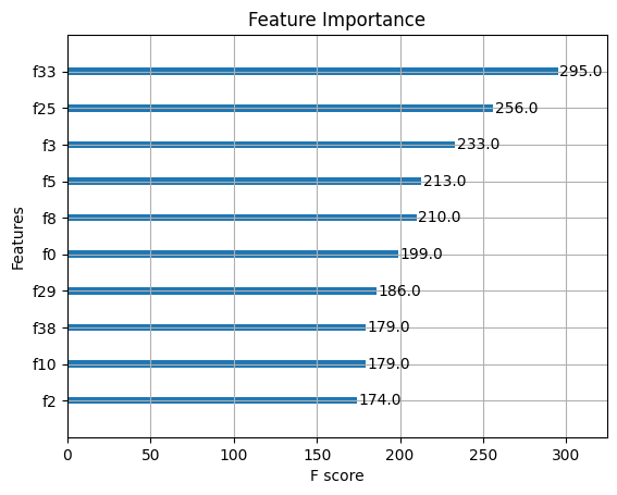
Now we will evaluate the performance of the model. In this step we have calculated the metrics like accuracy, precision recall etc. To further evaluate the performance we have also plotted confusion matrix and feature importance graph using Matplotlib and Seaborn. The feature importance graph is basically used to highlight which feature has been given more importance.
Python `
Calculate accuracy
accuracy = accuracy_score(y_test_encoded, y_pred) print(f'Accuracy: {accuracy:.2f}')
Print classification report
print(classification_report(y_test_encoded, y_pred, target_names=label_encoder.classes_))
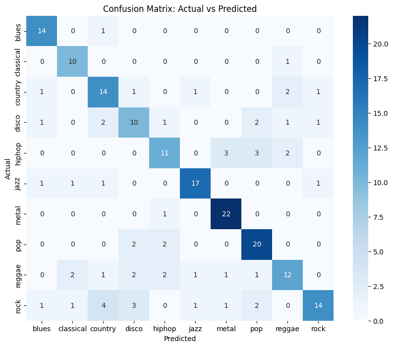
Confusion Matrix Visualization
conf_matrix = confusion_matrix(y_test_encoded, y_pred) plt.figure(figsize=(10, 8)) sns.heatmap(conf_matrix, annot=True, fmt='d', cmap='Blues', xticklabels=label_encoder.classes_, yticklabels=label_encoder.classes_) plt.ylabel('Actual') plt.xlabel('Predicted') plt.title('Confusion Matrix: Actual vs Predicted') plt.show()
Plot Feature Importance
plt.figure(figsize=(12, 10)) plot_importance(model, max_num_features=10, importance_type='weight') # Adjust max_num_features as needed plt.title('Feature Importance') plt.show()
`
**Output:
Accuracy: 0.72
precision recall f1-score support
blues 0.78 0.93 0.85 15 classical 0.71 0.91 0.80 11
country 0.61 0.70 0.65 20
disco 0.56 0.56 0.56 18
hiphop 0.65 0.58 0.61 19
jazz 0.85 0.81 0.83 21
metal 0.81 0.96 0.88 23
pop 0.71 0.83 0.77 24
reggae 0.67 0.55 0.60 22
rock 0.82 0.52 0.64 27
accuracy 0.72 200 macro avg 0.72 0.73 0.72 200
weighted avg 0.72 0.72 0.71 200
The accuracy of our model is 72% which is pretty good especially for music genre classification. For hiphop and reggae we can see that there is slight dip in the metrics. For other genres like rock, reggae there is dip in recall which highlights the fact that False Negatives is more.
**Below is the Confusion matrix and Feature Importance:
Automated Music Genre Classification
Automated Music Genre Classification
**Challenges and Future Directions
While automated music genre classification has made significant progress with the advent of deep learning techniques like CNNs, several challenges remain:
- **Genre Overlap: Many songs exhibit characteristics of multiple genres simultaneously.
- **Dataset Bias: The performance of models heavily depends on the quality and diversity of training datasets.
- **Real-time Processing: Developing models that can classify genres in real-time remains an ongoing challenge.
Conclusion
Librosa is a powerful library as it has the capability to capture the features of any audio. Using the mathematical techniques and transformation series like Fourier Transform, it has the capacity to highlight wide variety of features. With the help of Ensemble Learning techniques, we can easily classify the genres.