Parkinson Disease Prediction using Machine Learning Python (original) (raw)
Last Updated : 23 Jul, 2025
Parkinson's disease is a progressive neurological disorder that affects movement. Stiffening, tremors and slowing down of movements may be signs of Parkinson's disease. While there is no certain diagnostic test, but we can use machine learning in predicting whether a person has Parkinson's disease based on specific biomarkers. In this article, we will use machine learning models to predict Parkinson's disease.
1. Importing Libraries and Dataset
We will be using**Pandas, **Numpy, **Matplotlib, **Seaborn, **Sckit-learn, **XGBoost and **Imblearn.
Python `
import numpy as np import pandas as pd import matplotlib.pyplot as plt import seaborn as sb
from imblearn.over_sampling import RandomOverSampler from sklearn.model_selection import train_test_split from sklearn.preprocessing import LabelEncoder, MinMaxScaler from sklearn.feature_selection import SelectKBest, chi2 from tqdm.notebook import tqdm from sklearn import metrics from sklearn.svm import SVC from xgboost import XGBClassifier from sklearn.linear_model import LogisticRegression
import warnings warnings.filterwarnings('ignore')
`
2. Importing Dataset
The dataset we are going to use here includes 755 columns and three observations for each patient. The value's in these columns are part of some other diagnostics which are generally used to capture the difference between a healthy and affected person. Now, let's load the dataset into the panda's data frame. You can download dataset from here: Parkinson Disease Dataset.
Python `
df = pd.read_csv('parkinson_disease.csv') pd.set_option('display.max_columns', 10) df.sample(5)
`
**Output:
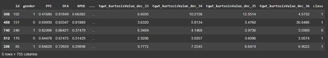
sample entries in the dataset
3. Data Exploration and Cleaning
To understand the dataset better we use some built-in functions from the **Pandas library. These functions help us inspect the structure, data types and statistical properties of the dataset.
df.info(): Displays the total number of rows and columns, the data types of each column and the count of non-null values. This helps identify missing data and column types.df.describe().T: Provides a transposed statistical summary of numerical columns, including the **mean, standard deviation, minimum and maximum values as well as quartiles. This helps us understand the distribution of the data.df.isnull().sum().sum(): Checks the total number of missing values in the dataset. If this returns **0 it means there are no missing values. If there are any null/missing values then we start with the data cleaning process to handle those values. Python `
df.info()
`
**Output:
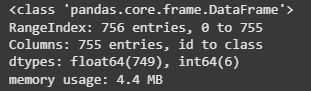
Information regarding data in the columns
Python `
df.describe().T
`
**Output:
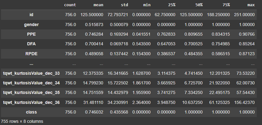
Descriptive statistical measures of the dataset
Python `
df.isnull().sum().sum()
`
**Output:
np.int64(0)
Therefore from the above analysis we concluded that our dataset contains no null/missing values and how the data is distributed in the given columns. Since there are no null/missing values there is no need for data cleaning.
4. Data Wrangling
Data wrangling involves restructuring and transforming the dataset to make it suitable for analysis. Since our dataset contains three observations for each patient we need to aggregate them to create a single representative record per patient. Here:
df.groupby('id').mean().reset_index(): Groups the dataset by the "id"column and calculates the mean of numerical features. This helps in aggregating multiple records of the sameid(patient id).df.drop('id', axis=1, inplace=True): Removes the "id"column as it is no longer needed after aggregation. Python `
df = df.groupby('id').mean().reset_index() df.drop('id', axis=1, inplace=True)
`
Multicollinearity can negatively impact machine learning models by making them unstable and less interpretable. To handle this we identify and remove highly correlated features from our dataset. In this code:
df[col].corr(df[col1]): Computes the Pearson correlation coefficient between two numerical features.- **If correlation > 0.7: The feature is considered highly correlated and is removed from the dataset to reduce redundancy.
- **The
classcolumn is excluded: Since it represents the target variable, we do not check its correlation with other features. Python `
columns = list(df.columns) for col in columns: if col == 'class': continue
filtered_columns = [col]
for col1 in df.columns:
    if((col == col1) | (col == 'class')):
        continue

    val = df[col].corr(df[col1])
    if val > 0.7:
        # If the correlation between the two features is more than 0.7, remove it
        columns.remove(col1)
        continue
    else:
        filtered_columns.append(col1)

df = df[filtered_columns]
df.shape
`
**Output:
(252, 287)
Now we can see that the dataset contained **755 features but after removing highly correlated ones the feature space was reduced to **287 columns. However this is still significantly high as the number of features **exceeds the number of data points (252 examples).
5. Feature Selection
To improve model performance and reduce computational complexity we apply **feature selection using the **chi-square test to retain only the most relevant features. This helps eliminate redundant or less significant variables making the dataset more efficient for machine learning. Here:
X = df.drop('class', axis=1): Extracts the feature set by removing the target variable (class).MinMaxScaler().fit_transform(X): Normalizes the feature values to a range of **[0,1] using **Min-Max Scaling. This ensures that all features contribute equally to the model.SelectKBest(chi2, k=30): Applies the **Chi-Square test to select the **30 most important features based on their relationship with the target variable (class).selector.fit(X_norm, df['class']): Fits the feature selection model on the normalized data.filtered_columns = selector.get_support(): Identifies the selected features.filtered_data = X.loc[:, filtered_columns]: Extracts only the top 30 selected features.filtered_data['class'] = df['class']: Reattaches the target variable (class) to the reduced dataset. Python `
X = df.drop('class', axis=1) X_norm = MinMaxScaler().fit_transform(X) selector = SelectKBest(chi2, k=30) selector.fit(X_norm, df['class']) filtered_columns = selector.get_support() filtered_data = X.loc[:, filtered_columns] filtered_data['class'] = df['class'] df = filtered_data df.shape
`
**Output:
(252, 31)
Therefore we reduce the dimensionality of our dataset by 30 since 1 is "class" column, while preserving the most important features making our dataset more efficient for model training.
6. Handling Class Imbalance and Splitting Data
To understand the distribution of target classes in our dataset, we use a **pie chart. This helps us check for class imbalances, which can impact model performance.
df['class'].value_counts(): Counts the occurrences of each class in the dataset.plt.pie(x.values, labels=x.index, autopct='%1.1f%%'): Creates a **pie chartx.values: Represents the frequency of each class.labels=x.index: Assigns class labels to each slice.autopct='%1.1f%%': Displays percentages with one decimal place.
This visualization helps us assess whether the dataset is **balanced or imbalanced which is crucial when selecting appropriate evaluation metrics and model strategies
Python `
x = df['class'].value_counts() plt.pie(x.values, labels = x.index, autopct='%1.1f%%') plt.show()
`
**Output:
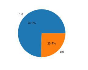
Pie chart for the distribution of the data within two class
To build a robust machine learning model we need to **address this **class imbalance and properly split the dataset into training and validation sets. If the dataset is imbalanced the model may become biased toward the majority class making it difficult to correctly predict the minority class. Here: ****:**
features = df.drop('class', axis=1): Extracts and stores independent variables.target = df['class']: Stores the dependent variable.****:**train_test_split(features, target, test_size=0.2, random_state=10): Allocates 80% of data for training and 20% for validationrandom_state=10ensures reproducibility.ros = RandomOverSampler(sampling_strategy='minority', random_state=0): Oversamples the minority class ensuring both classes have equal representation.ros.fit_resample(X_train, Y_train): Applies oversampling to the training dataset. Python `
features = df.drop('class', axis=1) target = df['class']
X_train, X_val,Y_train, Y_val = train_test_split(features, target, test_size=0.2, random_state=10)
ros = RandomOverSampler(sampling_strategy=1.0, random_state=0) X, Y = ros.fit_resample(X_train, Y_train) X.shape, Y.value_counts()
`
**Output:
((302, 30),
class
1.0 151
0.0 151
Name: count, dtype: int64)
By performing oversampling we created a balanced dataset preventing model bias toward the majority class making it more accurate on unseen data .
7. Model Training and Evaluation
After preparing the dataset, we train multiple machine learning models and evaluate their performance using the **ROC AUC Score. This helps us compare different models and choose the best-performing one for our classification task. Here we are using three different classifiers : **Logistic Regression, **XGBoost Classifier and **Support Vector Classifier****.**
model.fit(X_resampled, y_resampled: Trains each model in the "models" list .model.predict(X_resampled): Predicts outcomes on the training data.ras(y_resampled, train_preds): Computes the ROC AUC score for training accuracy.model.predict(X_val): Predicts outcomes on the validation dataset.ras(y_val, val_preds): Computes the ROC AUC score for validation accuracy. Python `
from sklearn.metrics import roc_auc_score as ras
models = [LogisticRegression(class_weight='balanced'), XGBClassifier(), SVC(kernel='rbf', probability=True)] for model in models: model.fit(X_resampled, y_resampled) print(f'{model} : ')
train_preds = model.predict(X_resampled)
print('Training Accuracy : ', ras(y_resampled, train_preds))

val_preds = model.predict(X_val)
print('Validation Accuracy : ', ras(y_val, val_preds))
print()
`
**Output:
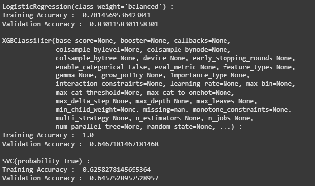
Model Training
From the above output we can say that Logistic Regression classifier performs better on the validation data with less difference between the validation and training data.
8. Analyzing Model Performance
We will now plot confusion matrix on validation data) for the Logistic Regression model to further evaluate the model's predictive capability.
ConfusionMatrixDisplay.from_estimator(models[0], X_val, y_val): Uses the first model in the list (which is Logistic Regression) to make predictions on the validation set (X_val).- It then compares these predictions to the actual labels
y_valto generate a confusion matrix. Python `
from sklearn.metrics import ConfusionMatrixDisplay
ConfusionMatrixDisplay.from_estimator(models[0], X_val, Y_val) plt.show()
`
**Output:

Confusion matrix for the validation data
Upon analyzing this confusion matrix we are able to conclude that :
- **True Positives (TP) = 35 : The model correctly predicted 35 healthy individuals.
- **True Negatives (TN) = 10 : The model correctly predicted 10 unhealthy individuals.
- **False Positives (FP) = 4 : The model incorrectly classified 4 unhealthy individuals as healthy.
- **False Negatives (FN) = 2 : The model incorrectly classified 2 healthy individuals as unhealthy.
This analysis concludes that the model correctly classifies most cases but still misclassified a few unhealthy patients (FN = 2) . We will now plot the classification report for the Logistic Regression Classifier model.
Python `
from sklearn.metrics import classification_report print(classification_report(y_val, models[0].predict(X_val)))
`
**Output:
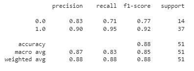
classification report
This report indicates that the model performs well overall, particularly in detecting healthy individuals. However there is room for improvement in recall for the unhealthy class (0.71) suggesting that the model sometimes fails to correctly identify unhealthy individuals.
You can download the source code from here : Parkinson Disease Prediction using Machine Learning.