SHAP : A Comprehensive Guide to SHapley Additive exPlanations (original) (raw)
Last Updated : 14 Jul, 2025
Interpreting models is an important part of machine learning, especially when dealing with black-box models like XGBoost or deep neural networks. SHAP (SHapley Additive exPlanations) provides a robust and sound method to interpret model predictions by making attributes of importance scores to input features.
What is SHAP?
SHAP is a method that helps us understand how a machine learning model makes decisions. It tells us how much each input (feature) is helping or hurting the final prediction. The main idea is to fairly distribute the "payout" (the prediction) among all features based on their contribution.
Key Characteristics
- **Model-Agnostic: Works with any machine learning model.
- **Fair Attribution: Ensures consistent and fair distribution of feature importance.
- **Additive Feature Attribution: Sum of SHAP values equals the model prediction minus the baseline.
Unlike traditional feature importance techniques, SHAP provides local explanations (per prediction) in addition to global feature importance, making it more versatile.
SHAP with XGBoost Regression
We demonstrate SHAP with an XGBoost regression model trained on the Abalone dataset to predict the age of abalone based on physical characteristics.
**Step 1: Install Required Libraries
Python `
pip install xgboost shap pandas scikit-learn matplotlib ipywidgets
`
**Step 2: Load and Prepare the Dataset
- Load the Abalone dataset and assign column names.
- One-hot encode the categorical 'Sex' feature.
- Split the data into features (
X) and target (y= 'Rings'). - Divide the dataset into training and test sets (80/20 split). Python `
import pandas as pd from sklearn.model_selection import train_test_split import xgboost as xgb
file_path = "SHAP_ex.txt" # Replace with your actual file path columns = ["Sex", "Length", "Diameter", "Height", "WholeWeight", "ShuckedWeight", "VisceraWeight", "ShellWeight", "Rings"] abalone = pd.read_csv(file_path, header=None, names=columns)
One-hot encode 'Sex' and separate features
X = pd.get_dummies(abalone.drop("Rings", axis=1), columns=["Sex"], drop_first=True) y = abalone["Rings"]
Split data
X_train, X_test, y_train, y_test = train_test_split(X, y, test_size=0.2, random_state=42)
`
**Step 3: Train the XGBoost Regressor
- model = xgb.XGBRegressor(): Creates an XGBoost regression model object.
- model.fit(X_train, y_train): Trains the model using the training data (X_train and y_train). Python `
model = xgb.XGBRegressor() model.fit(X_train, y_train)
`
SHAP Explanation and Visualizations
**Step 4: Initialize the SHAP Explainer
- import shap: Imports the SHAP library for model interpretation.
- explainer = shap.Explainer(model): Creates a SHAP explainer for the trained model.
- shap_values = explainer(X_test): Computes SHAP values for the test data to explain predictions.
- shap.initjs(): Initializes JavaScript support for SHAP visualizations in notebooks. Python `
import shap explainer = shap.Explainer(model) shap_values = explainer(X_test) shap.initjs()
`
SHAP (SHapley Additive exPlanations) has a variety of visualization tools that help interpret machine learning model predictions. These plots highlight which features are important and also explain how they influence individual or overall model outputs. Below are some commonly used SHAP visualizations and what they reveal about model behavior:
**4.1 Waterfall Model
Shows how each feature contributes to the difference between the model's base value and the output prediction for a specific instance.
Python `
shap.waterfall_plot(shap_values[0])
`
**Output:
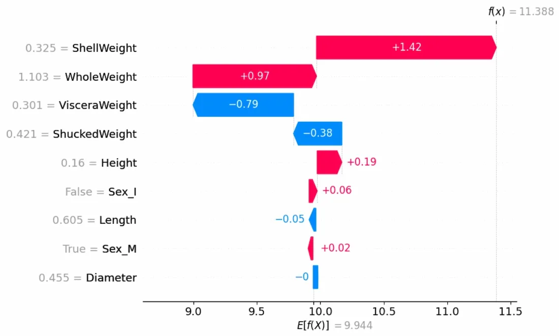
Waterfall Plot
**Color Guide:
- **Red = pushes prediction higher
- **Blue = pushes prediction lower
**4.2 Force Plot
Gives an interactive view of individual prediction explanations.
Python `
shap.force_plot(explainer.expected_value, shap_values[0].values, X_test.iloc[0, :], matplotlib=True)
`
**Output:
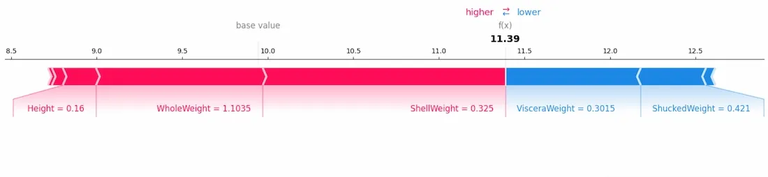
Force Plot
This plot displays the positive and negative influences of features in a linear format.
**4.3 Stacked Force Plot
Visualizes feature contributions across multiple observations.
Python `
for i in range(100): shap.force_plot(explainer.expected_value, shap_values[i].values, X_test.iloc[i, :], matplotlib=True)
`
**Output:
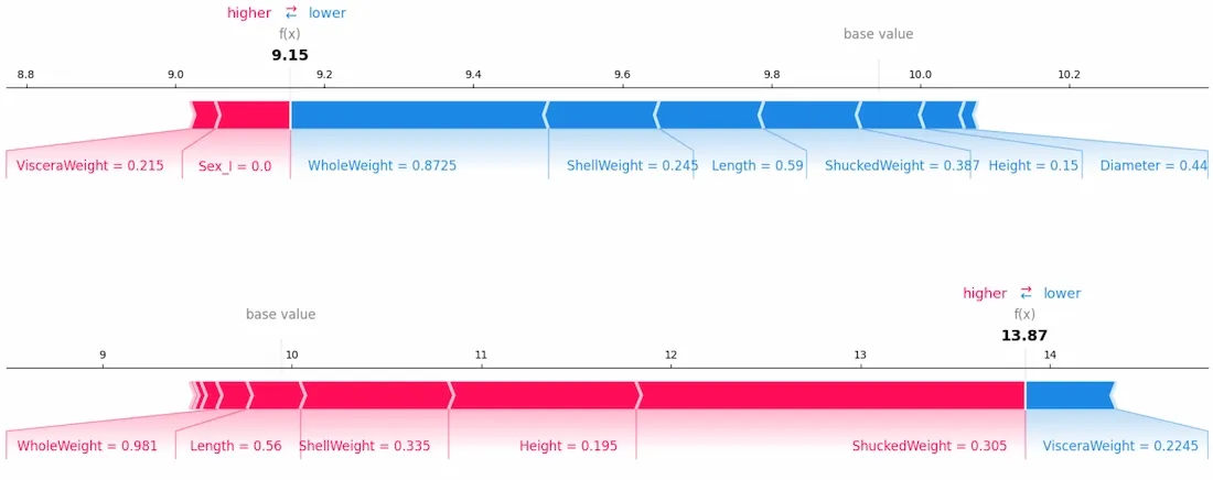
Stacked Force plot
4.4 **Summary Plot
Gives a global view of feature importance and how values influence predictions.
Python `
shap.summary_plot(shap_values, X_test)
`
**Output:
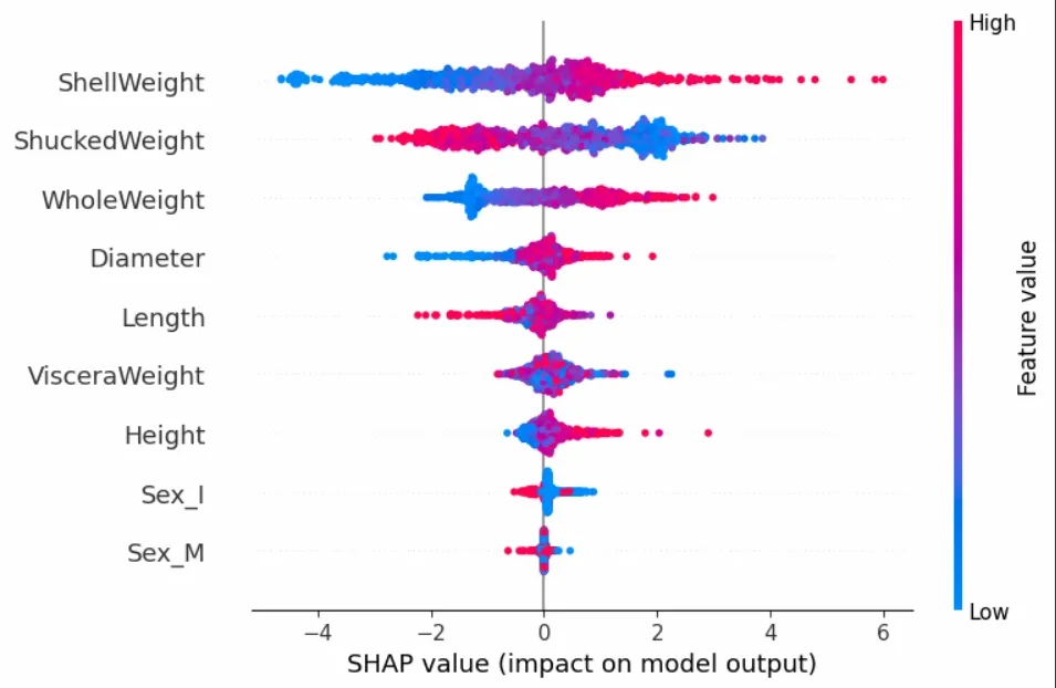
Summary Plot
- Horizontal location shows whether the effect of that value is associated with a higher or lower prediction.
- Color represents the original value of the feature.
**4.5 Bar Plot of Mean SHAP Values
Displays average feature impact across the dataset.
Python `
shap.summary_plot(shap_values, X_test, plot_type="bar")
`
**Output:
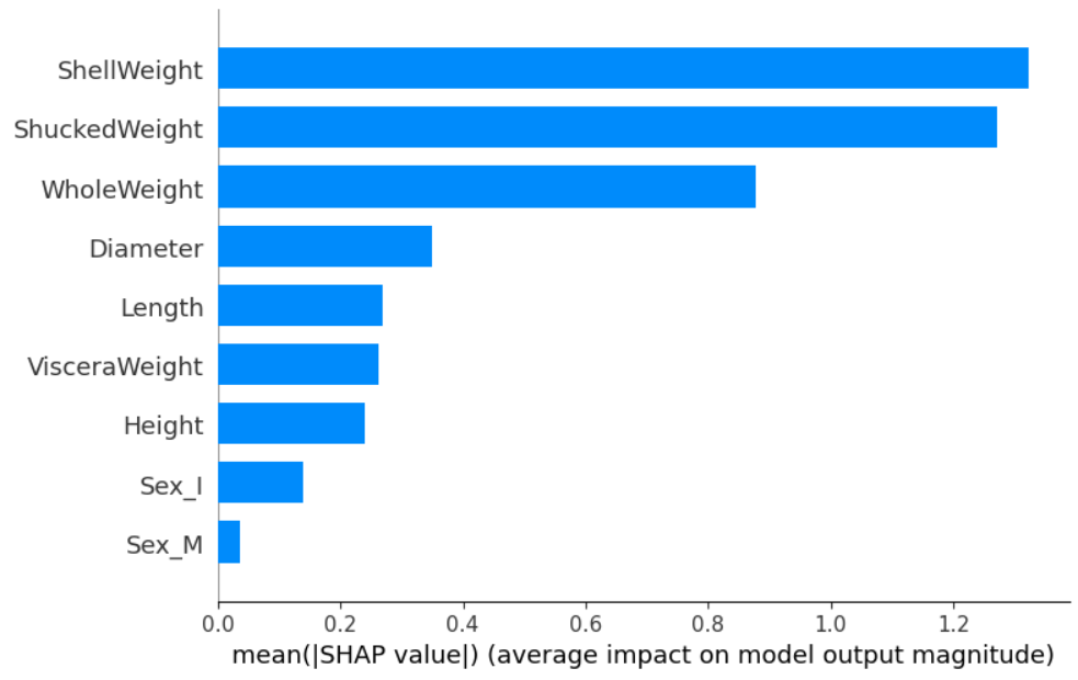
Bar plot of mean SHAP values
This is helpful when identifying which features are generally more important.
**4.6 Dependence Plot
Shows how the SHAP value of a single feature varies with its value.
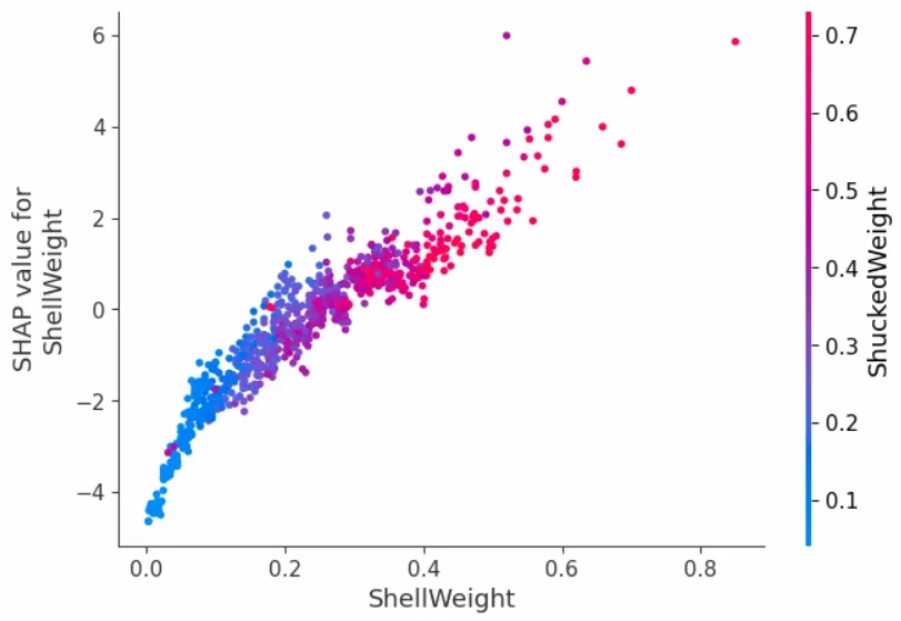
Dependance Plot
This helps capture feature interactions as well.
Interpreting Black Box Models
SHAP also supports interpretation of other models like decision trees, random forests, or even neural networks.
Example with Decision Tree Classifier on Iris Dataset
- Loads the Iris dataset with features of different flower species.
- Splits the data into training and test sets.
- Trains a DecisionTreeClassifier on the training data.
- Uses SHAP to explain how each feature affects model predictions.
- Displays a summary plot to show feature importance and their influence on predictions. Python `
from sklearn.datasets import load_iris from sklearn.tree import DecisionTreeClassifier
iris = load_iris() X = pd.DataFrame(iris.data, columns=iris.feature_names) y = pd.Series(iris.target)
X_train, X_test, y_train, y_test = train_test_split(X, y, random_state=42)
clf = DecisionTreeClassifier(random_state=42) clf.fit(X_train, y_train)
explainer = shap.Explainer(clf) shap_values = explainer(X_test)
shap.summary_plot(shap_values, X_test)
`
**Output:
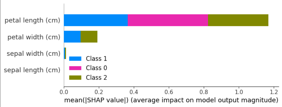
SHAP over Decision tree model
This example shows that SHAP can effectively interpret predictions from even simple models like decision trees, making it a tool for understanding both black-box and transparent models across a wide range of machine learning applications.
Benefits of SHAP
- **Model Interpretability: Makes ML models transparent by explaining predictions.
- **Fairness Audits: Helps detect bias in model decisions.
- **Model Debugging: Useful during error analysis or model tuning.
- **Universality: Compatible with tree-based, linear, and deep learning models.
Challenges of Using SHAP
| Challenge | Description |
|---|---|
| Computational Overhead | Can be slow for large datasets or complex models |
| High-Dimensional Data | Visualization and computation become difficult |
| Model-Dependent Behavior | Interpretation may vary across different models |
| Resource Consumption | Requires additional time and memory |
| Input Sensitivity | Can be sensitive to feature correlation or data order |
In summary, SHAP is a powerful tool that helps us see which parts of our data matter the most in making predictions. It works for different kinds of models and shows us clear pictures to make things easier to understand. This makes it really useful for people who want to better understand their complicated models.
Related Articles
Python
- Leveraging SHAP values for Model Insights
- SHAP with a linear SVC model
- Feature Importance in Random Forests