Lasso Regression in R Programming (original) (raw)
Last Updated : 9 Jul, 2025
Lasso Regression is a linear modeling technique that uses L1 regularization to improve prediction accuracy and model interpretability. By adding a penalty equal to the absolute values of the coefficients, it shrinks some of them to zero, effectively performing feature selection and reducing model complexity, especially in high-dimensional data.
Key Characteristics
- Performs both regularization and feature selection.
- Suitable for high-dimensional data.
- Helps reduce variance while possibly increasing bias slightly.
- Works well when there are many correlated features.
Mathematical Formulation
The cost function minimized by Lasso Regression is:
\text{min} \left( \frac{1}{2N} \sum_{i=1}^{N} (y_i - \beta_0 - \sum_{j=1}^{p} x_{ij}\beta_j)^2 + \lambda \sum_{j=1}^{p} |\beta_j| \right)
**Where:
- N : number of observations
- p****:** number of predictors
- y_i ****:** actual output
- x_{ij} : input features
- \beta_0 : intercept term
- \beta_j ****:** model coefficients
- \lambda: regularization strength
Effect of Lambda (λ)
- \lambda=0: Equivalent to ordinary least squares regression.
- **As \lambda increases: More coefficients shrink to exactly zero, enhancing feature selection.
- **Very high \lambda : All coefficients become zero, leading to underfitting.
Implementation of Lasso Regression in R
We implement Lasso Regression using the Big Mart Sales dataset, aiming to predict product sales based on various product and outlet features. The process involves data preprocessing, encoding, normalization and training using the glmnet package with L1 regularization.
1. Installing Required Packages
We install the necessary packages to preprocess data, train the Lasso regression model and visualize results.
- **data.table: used for efficient data loading and manipulation.
- **dplyr: used for data transformation and filtering.
- **glmnet: used for fitting Lasso and Ridge regression models.
- **ggplot2: used for plotting and visualization.
- **caret: used to train and tune models using cross-validation.
- **xgboost: used for ensemble tree-based models.
- **e1071: used for statistical measures like skewness.
- **cowplot: used to arrange multiple plots together. R `
install.packages("data.table") install.packages("dplyr") install.packages("glmnet") install.packages("ggplot2") install.packages("caret") install.packages("xgboost") install.packages("e1071") install.packages("cowplot")
library(data.table) library(dplyr) library(glmnet) library(ggplot2) library(caret) library(xgboost) library(e1071) library(cowplot)
`
2. Loading and Combining the Dataset
We load and merge the train and test datasets to perform uniform preprocessing on the entire data.
You can download the dataset from here: Train.csv and Test.csv.
- **fread: used to load CSV data efficiently.
- **rbind: used to merge two datasets row-wise.
- ****:=**: used to add or modify columns in a data.table. R `
train = fread("Train.csv") test = fread("Test.csv") test[, Item_Outlet_Sales := NA] combi = rbind(train, test)
`
3. Treating Missing and Zero Values
We handle missing weights and zero visibility values by imputing with mean values.
- **which: used to identify indices of NA or zero values.
- **mean: used to compute average values for imputation. R `
missing_index = which(is.na(combi$Item_Weight)) for(i in missing_index) { item = combi$Item_Identifier[i] combi$Item_Weight[i] = mean(combi$Item_Weight[combi$Item_Identifier == item], na.rm = TRUE) }
zero_index = which(combi$Item_Visibility == 0) for(i in zero_index) { item = combi$Item_Identifier[i] combi$Item_Visibility[i] = mean(combi$Item_Visibility[combi$Item_Identifier == item], na.rm = TRUE) }
`
4. Encoding Categorical Features
We convert categorical variables into numeric form using label encoding and one-hot encoding.
- **ifelse: used for conditional numeric transformation.
- **dummyVars: used to generate one-hot encoded columns.
- **predict: used to apply transformations from dummyVars. R `
combi[, Outlet_Size_num := ifelse(Outlet_Size == "Small", 0, ifelse(Outlet_Size == "Medium", 1, 2))] combi[, Outlet_Location_Type_num := ifelse(Outlet_Location_Type == "Tier 3", 0, ifelse(Outlet_Location_Type == "Tier 2", 1, 2))] combi[, c("Outlet_Size", "Outlet_Location_Type") := NULL]
ohe_1 = dummyVars("~.", data = combi[, -c("Item_Identifier", "Outlet_Establishment_Year", "Item_Type")], fullRank = TRUE) ohe_df = data.table(predict(ohe_1, combi[, -c("Item_Identifier", "Outlet_Establishment_Year", "Item_Type")])) combi = cbind(combi[, "Item_Identifier"], ohe_df)
`
5. Transforming and Scaling Features
We reduce skewness and standardize numeric features to improve model performance.
- **log: used to reduce skewness by logarithmic transformation.
- **sapply: used to apply functions across columns.
- **preProcess: used for centering and scaling features. R `
combi[, Item_Visibility := log(Item_Visibility + 1)]
num_vars = which(sapply(combi, is.numeric)) num_vars_names = names(num_vars) combi_numeric = combi[, setdiff(num_vars_names, "Item_Outlet_Sales"), with = FALSE]
prep_num = preProcess(combi_numeric, method = c("center", "scale")) combi_numeric_norm = predict(prep_num, combi_numeric)
combi[, setdiff(num_vars_names, "Item_Outlet_Sales") := NULL] combi = cbind(combi, combi_numeric_norm)
`
6. Splitting the Data
We split the processed combined data back into separate train and test sets.
- **nrow: used to calculate number of rows for splitting.
- ****:= NULL**: used to delete a column. R `
train = combi[1:nrow(train)] test = combi[(nrow(train) + 1):nrow(combi)] test[, Item_Outlet_Sales := NULL]
`
7. Training Lasso Regression Model
We train the model using cross-validation and tune the lambda regularization parameter.
- **trainControl: used to define cross-validation settings.
- **expand.grid: used to specify tuning parameter grid.
- **train: used to train the model with given tuning strategy.
- **mean: used to compute average validation RMSE. R `
set.seed(123) control = trainControl(method = "cv", number = 5) Grid_la_reg = expand.grid(alpha = 1, lambda = seq(0.001, 0.1, by = 0.0002))
lasso_model = train(x = train[, -c("Item_Identifier", "Item_Outlet_Sales")], y = train$Item_Outlet_Sales, method = "glmnet", trControl = control, tuneGrid = Grid_la_reg)
cat("Mean validation test =", mean(lasso_model$resample$RMSE))
`
**Output:
Mean validation test = 1129.059
8. Visualizing Lasso Model Coefficients
We extract and plot the non-zero coefficients from the final trained Lasso model to interpret the influence of features.
- **coef: used to extract the fitted coefficients from the model object.
- **as.matrix: used to convert the sparse coefficient object to a standard matrix.
- **rownames: used to extract feature names.
- **theme(axis.text.x = …): used to rotate axis labels. R `
lasso_coefs = as.matrix(coef(lasso_model$finalModel, s = lasso_model$bestTune$lambda)) lasso_coefs_df = data.frame( Predictor = rownames(lasso_coefs), Coefficient = as.numeric(lasso_coefs) ) lasso_coefs_df = lasso_coefs_df[lasso_coefs_df$Predictor != "(Intercept)" & lasso_coefs_df$Coefficient != 0, ]
ggplot(lasso_coefs_df, aes(x = reorder(Predictor, Coefficient), y = Coefficient)) + geom_bar(stat = "identity", fill = "skyblue", color = "black") + labs(title = "Lasso Regression Coefficients", x = "Predictor", y = "Coefficient") + theme_minimal() + theme(axis.text.x = element_text(angle = 45, hjust = 1))
`
**Output:
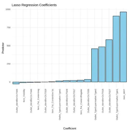
Output
The plot displays the non-zero coefficients from a Lasso regression model, highlighting the most influential features on the target variable. Item_MRP and Outlet_Type_Supermarket_Type1 have the highest positive impact, while several features have coefficients close to zero, indicating minimal or no contribution.
Applications of Lasso Regression
- **Feature selection: Ideal for reducing overfitting by selecting only the most relevant variables.
- **High-dimensional modeling: Useful when number of predictors exceeds number of observations.
- **Finance: Used in credit risk models where many financial indicators exist.
- **Genomics: Applied to select key genes in DNA analysis.
- **Retail forecasting: Filters product/store features for effective sales prediction.