Parametric Tests in R (original) (raw)
Last Updated : 12 Jul, 2025
In R, a parametric test is a statistical method that makes specific assumptions about the population distribution, often assuming normality, equal variance and interval or ratio scale. These tests are typically more powerful when assumptions are satisfied and are widely used in hypothesis testing, mean comparisons and variance analysis.
Common Parametric Tests in R
R provides several parametric tests used when the data meet the assumptions required for parametric methods. These tests are suitable for normally distributed, continuous and interval-scale data.
1. T-Test
The T-Test in R is used to compare means and test hypotheses about population means. It assumes the data is approximately normally distributed and comes in three main forms: one-sample, two-sample (independent) and paired t-test.
**1.1 One-Sample t-Test
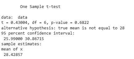
The One-Sample t-Test is used to check if the mean of a sample is different from a known or hypothesized value.
**Syntax:
t.test(x, mu = value)
- **t.test(): Used to perform one and two sample t-tests on vector data. The mu argument specifies the hypothesized mean.
**Example: The One-Sample t-Test checks if the mean of a given sample is equal to 28. We are testing whether the sample’s mean is different from 28.
R `
data <- c(25, 27, 26, 30, 28, 32, 31) result <- t.test(data, mu = 28) print(result)
`
**Output:
Output
**1.2 Two-Sample t-Test (Independent t-Test)
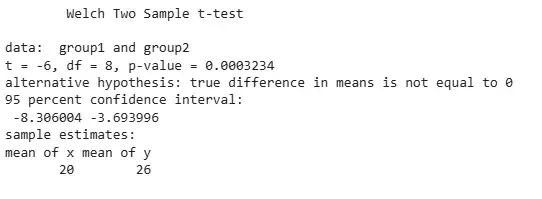
The Two-Sample t-Test is used to compare the means of two independent groups. It assumes equal variances and normal distribution.
**Syntax:
t.test(x, y)
- **t.test(): Used to compare the means of two independent groups. The vectors
xandyrepresent the two groups.
**Example: The Two-Sample t-Test compares the means of group1 and group2 to see if they are different.
R `
group1 <- c(18, 22, 19, 21, 20) group2 <- c(25, 27, 24, 26, 28) result <- t.test(group1, group2) print(result)
`
**Output:
Output
**1.3 Paired t-Test
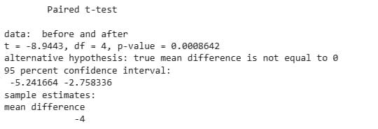
The Paired t-Test is used to compare means from the same group at different times or under two different conditions.
**Syntax:
t.test(x, y, paired = TRUE)
- **t.test(): When paired = TRUE, it performs a paired t-test comparing two related samples (e.g., before and after treatment).
**Example: The Paired t-Test compares before and after values to test if there is a significant difference between them.
R `
before <- c(55, 60, 58, 62, 59) after <- c(60, 63, 62, 65, 64) result <- t.test(before, after, paired = TRUE) print(result)
`
**Output:
Output
2. ANOVA (Analysis of Variance)
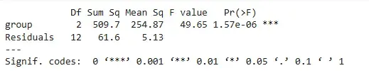
The ANOVA test is used to compare the means of three or more independent groups to determine if there are any statistically significant differences.
**Syntax:
aov(response ~ factor, data = dataset)
- **aov(): Used to perform analysis of variance (ANOVA), comparing means across multiple groups using a formula interface.
Example: The ANOVA test compares scores across three groups A, B and C to check for any differences.
R `
group <- factor(rep(c("A", "B", "C"), each = 5)) scores <- c(80, 85, 82, 88, 84, 90, 92, 95, 91, 93, 78, 76, 80, 79, 77) result <- aov(scores ~ group) summary(result)
`
**Output:
Output
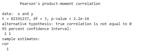
3. Pearson Correlation Test
The Pearson Correlation Test is used to assess the strength and direction of the linear relationship between two continuous variables.
**Syntax:
cor.test(x, y, method = "pearson")
- **cor.test(): Computes the correlation coefficient between two variables. When method = "pearson", it performs a Pearson correlation test.
**Example: The Pearson Correlation Test measures the linear correlation between variables x and y.
R `
x <- c(1, 2, 3, 4, 5) y <- c(2, 4, 6, 8, 10) result <- cor.test(x, y, method = "pearson") print(result)
`
**Output:
Output
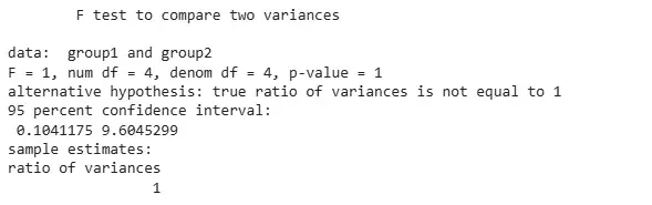
4. F-Test
The F-Test is used to compare the variances of two samples to determine if they are different.
**Syntax:
var.test(x, y)
- **var.test(): Performs an F-test to compare the variances of two groups. The two numeric vectors
xandyrepresent the samples.
**Example: The F-Test checks if group1 and group2 have equal variances.
R `
group1 <- c(15, 18, 17, 16, 19) group2 <- c(22, 25, 24, 26, 23) result <- var.test(group1, group2) print(result)
`
**Output:
Output
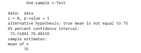
5. Z-Test
The Z-Test is used to determine whether there is a difference between sample and population means when the population variance is known and the sample size is large (n > 30).
**Syntax:
BSDA::z.test(x, mu = value, sigma.x = sd)
- **z.test(): Performs a Z-Test. Requires population standard deviation sigma.x and hypothesized mean mu. Part of the BSDA package.
**Example: The Z-Test checks if the mean of the sample differs significantly from 75, assuming known population standard deviation.
R `
library(BSDA) data <- c(72, 74, 76, 78, 75, 77, 73) result <- z.test(data, mu = 75, sigma.x = 2) print(result)
`
**Output:
Output
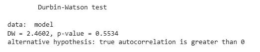
6. Durbin-Watson Test
The Durbin-Watson Test is used to detect the presence of autocorrelation in the residuals from a regression analysis.
**Syntax:
lmtest::dwtest(model)
- **dwtest(): Performs the Durbin-Watson test on a linear model to check for autocorrelation in residuals. Part of the lmtest package.
Example: The Durbin-Watson Test checks for autocorrelation in the residuals of a simple linear regression model.
R `
library(lmtest) x <- c(1, 2, 3, 4, 5, 6, 7) y <- c(2, 4, 6, 8, 10, 12, 14) model <- lm(y ~ x) result <- dwtest(model) print(result)
`
**Output:
Output
A Durbin-Watson statistic of 2.4602 with a p-value of 0.5534 indicates no positive autocorrelation in the residuals, so we fail to reject the null hypothesis.