Probabilities using R (original) (raw)

Last Updated : 24 Jul, 2025

Probability is the measure of the likelihood that a specific event will occur. It is expressed as a number between 0 and 1, where 0 means the event cannot happen and 1 means it will definitely happen. Probabilities are used to quantify uncertainty in experiments, real-world events and simulations. In R, we can calculate and visualize probabilities using built-in functions and packages.

Basic Concepts of Probability in R

• **Sample Space (S): The set of all possible outcomes of a random experiment.
• **Event: Any subset of the sample space.
• **Probability of an Event: The likelihood of occurrence of an event, calculated as the ratio of favorable outcomes to the total number of outcomes.

Calculating Probabilities in R

R offers various functions and packages for calculating Probability in R and performing statistical analyses. Some commonly used functions include:

• dbinom(): Computes the probability mass function (PMF) for the binomial distribution.
• pnorm(): Calculates the cumulative distribution function (CDF) for the normal distribution.
• dpois(): Computes the PMF for the Poisson distribution.
• punif(): Calculates the CDF for the uniform distribution.

**Example:

R `

sample_space <- c(1, 2, 3, 4, 5, 6) event <- c(2, 4, 6) probability <- length(event) / length(sample_space) print(probability)

`

**Output:

[1] 0.5

Probability Distributions in R

R provides extensive support for probability distributions, which are mathematical functions that describe the likelihood of different outcomes in a random experiment. Common probability distributions include:

• **Uniform Distribution:All outcomes are equally likely.
• **Normal Distribution: Symmetric bell-shaped curve, characterized by mean (μ) and standard deviation (σ).
• **Binomial Distribution: Describes the number of successes in a fixed number of independent Bernoulli trials.
• **Poisson Distribution: Models the number of events occurring in a fixed interval of time or space.

**Example:

R `

library(ggplot2)

x <- seq(-4, 4, length.out = 100) y <- dnorm(x, mean = 0, sd = 1)

df <- data.frame(x, y)

ggplot(df, aes(x = x, y = y)) + geom_line(color = "blue") + labs(title = "Normal Distribution", x = "x", y = "Density") + theme_minimal()

`

**Output:

Normal Distribution

Simulating Probabilistic Experiments in R

Simulation is a powerful tool for understanding probabilities through empirical experiments. R facilitates simulation by allowing the generation of random numbers from different probability distributions. Key functions for simulation include:

• runif(): Generates random numbers from a uniform distribution.
• rnorm(): Generates random numbers from a normal distribution.
• rbinom(): Generates random numbers from a binomial distribution.
• rpois(): Generates random numbers from a Poisson distribution. R `

num_flips <- 1000 num_heads <- sum(rbinom(num_flips, size = 1, prob = 0.5)) probability_heads <- num_heads / num_flips print(probability_heads)

`

**Output:

[1] 0.494

Visualizing Probabilities in R

Visualization is for gaining insights from Probability in R and it offers numerous packages such as ggplot2, lattice and base graphics for creating visualizations. Common plots include histograms, density plots, boxplots and scatter plots, which help in understanding the shape and characteristics of probability distributions.

R `

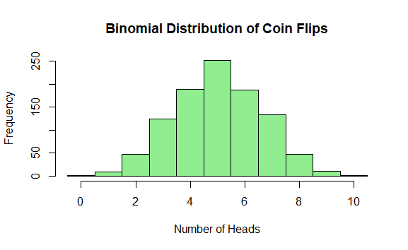
flips <- rbinom(1000, size = 10, prob = 0.5)

hist(flips, breaks = seq(-0.5, 10.5, by = 1), col = "lightgreen", main = "Binomial Distribution of Coin Flips", xlab = "Number of Heads", ylab = "Frequency")

`

**Output:

Probabilities using R

The output shows a histogram of the binomial distribution for 1000 trials of flipping a fair coin 10 times. Most results center around 5 heads, forming a symmetric, bell-shaped curve.