spectrogram - Spectrogram using short-time Fourier transform - MATLAB (original) (raw)

Spectrogram using short-time Fourier transform

Syntax

Description

[s](#bultmx7-s) = spectrogram([x](#bultmx7-x)) returns theShort-Time Fourier Transform (STFT) of the input signal x. Each column ofs contains an estimate of the short-term, time-localized frequency content of x. The magnitude squared of s is known as the_spectrogram_ time-frequency representation ofx [1].

example

[s](#bultmx7-s) = spectrogram([x](#bultmx7-x),[window](#bultmx7-window)) uses window to divide the signal into segments and perform windowing.

example

[s](#bultmx7-s) = spectrogram([x](#bultmx7-x),[window](#bultmx7-window),[noverlap](#bultmx7-noverlap)) uses noverlap samples of overlap between adjoining segments.

example

[s](#bultmx7-s) = spectrogram([x](#bultmx7-x),[window](#bultmx7-window),[noverlap](#bultmx7-noverlap),[nfft](#bultmx7-nfft)) uses nfft sampling points to calculate the discrete Fourier transform.

example

[[s](#bultmx7-s),[w](spectrogram.html#bultmx7-w),[t](spectrogram.html#bultmx7-t)] = spectrogram(___) returns a vector of normalized frequencies, w, and a vector of time instants, t, at which the STFT is computed. This syntax can include any combination of input arguments from previous syntaxes.

example

[[s](#bultmx7-s),[f](spectrogram.html#bultmx7-f-dup1),[t](spectrogram.html#bultmx7-t)] = spectrogram(___,[fs](#bultmx7-fs)) returns a vector of cyclical frequencies, f, expressed in terms of the sample rate fs. fs must be the fifth input to spectrogram. To input a sample rate and still use the default values of the preceding optional arguments, specify these arguments as empty, [].

example

[[s](#bultmx7-s),[w](spectrogram.html#bultmx7-w),[t](#bultmx7-t)] = spectrogram([x](#bultmx7-x),[window](#bultmx7-window),[noverlap](#bultmx7-noverlap),[w](spectrogram.html#bultmx7-w)) returns the STFT at the normalized frequencies specified in w. w must have at least two elements, because otherwise the function interprets it asnfft.

example

[[s](#bultmx7-s),[f](spectrogram.html#bultmx7-f-dup1),[t](#bultmx7-t)] = spectrogram([x](#bultmx7-x),[window](#bultmx7-window),[noverlap](#bultmx7-noverlap),[f](spectrogram.html#bultmx7-f),[fs](#bultmx7-fs)) returns the STFT at the cyclical frequencies specified in f. f must have at least two elements, because otherwise the function interprets it asnfft.

example

[___,[ps](#bultmx7-ps)] = spectrogram(___,[spectrumtype](#bultmx7-spectrumtype)) also returns a matrix, ps, proportional to the spectrogram of x.

• If you specify spectrumtype as"psd", each column of ps contains an estimate of the power spectral density (PSD) of a windowed segment.
• If you specify spectrumtype as"power", each column ofps contains an estimate of the power spectrum of a windowed segment.

example

[___] = spectrogram(___,"reassigned") reassigns each PSD or power spectrum estimate to the location of its center of energy. If your signal contains well-localized temporal or spectral components, then this option generates a sharper spectrogram.

example

[___,[ps](#bultmx7-ps),[fc](#bultmx7-fc),[tc](#bultmx7-fc)] = spectrogram(___) also returns two matrices, fc and tc, containing the frequency and time of the center of energy of each PSD or power spectrum estimate.

example

[___] = spectrogram(___,[freqrange](#bultmx7-freqrange)) returns the PSD or power spectrum estimate over the frequency range specified byfreqrange. Valid options forfreqrange are "onesided","twosided", and "centered".

example

[___] = spectrogram(___,[Name=Value](#namevaluepairarguments)) specifies additional options using name-value arguments. Options include the minimum threshold and output time dimension.

example

spectrogram(___) with no output arguments plotsps in decibels in the current figure window.

example

spectrogram(___,[freqloc](#bultmx7-freqloc)) specifies the axis on which to plot the frequency.

example

Examples

collapse all

Generate Nx=1024 samples of a signal that consists of a sum of sinusoids. The normalized frequencies of the sinusoids are 2π/5 rad/sample and 4π/5 rad/sample. The higher frequency sinusoid has 10 times the amplitude of the other sinusoid.

N = 1024; n = 0:N-1;

w0 = 2pi/5; x = sin(w0n)+10sin(2w0*n);

Compute the short-time Fourier transform using the function defaults. Plot the spectrogram.

s = spectrogram(x);

spectrogram(x,'yaxis')

Repeat the computation.

• Divide the signal into sections of length nsc=⌊Nx/4.5⌋.
• Window the sections using a Hamming window.
• Specify 50% overlap between contiguous sections.
• To compute the FFT, use max(256,2p) points, where p=⌈log2nsc⌉.

Verify that the two approaches give identical results.

Nx = length(x); nsc = floor(Nx/4.5); nov = floor(nsc/2); nff = max(256,2^nextpow2(nsc));

t = spectrogram(x,hamming(nsc),nov,nff);

maxerr = max(abs(abs(t(:))-abs(s(:))))

Divide the signal into 8 sections of equal length, with 50% overlap between sections. Specify the same FFT length as in the preceding step. Compute the short-time Fourier transform and verify that it gives the same result as the previous two procedures.

ns = 8; ov = 0.5; lsc = floor(Nx/(ns-(ns-1)*ov));

t = spectrogram(x,lsc,floor(ov*lsc),nff);

maxerr = max(abs(abs(t(:))-abs(s(:))))

Generate a signal that consists of a complex-valued convex quadratic chirp sampled at 600 Hz for 2 seconds. The chirp has an initial frequency of 250 Hz and a final frequency of 50 Hz.

fs = 6e2; ts = 0:1/fs:2; x = chirp(ts,250,ts(end),50,"quadratic",0,"convex","complex");

spectrogram Function

Use the spectrogram function to compute the STFT of the signal.

• Divide the signal into segments, each M=49 samples long.
• Specify L=11 samples of overlap between adjoining segments.
• Discard the final, shorter segment.
• Window each segment with a Bartlett window.
• Evaluate the discrete Fourier transform of each segment at NDFT=1024 points. By default, spectrogram computes two-sided transforms for complex-valued signals.

M = 49; L = 11; g = bartlett(M); Ndft = 1024;

[s,f,t] = spectrogram(x,g,L,Ndft,fs);

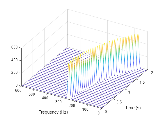
Use the waterplot function to compute and display the spectrogram, defined as the magnitude squared of the STFT.

STFT Definition

Compute the STFT of the Nx-sample signal using the definition. Divide the signal into ⌊Nx-LM-L⌋ overlapping segments. Window each segment and evaluate its discrete Fourier transform at NDFT points.

segs = framesig(1:length(x),M,OverlapLength=L); X = fft(x(segs).*g,Ndft);

Compute the time and frequency ranges for the STFT.

• To find the time values, divide the time vector into overlapping segments. The time values are the midpoints of the segments, with each segment treated as an interval open at the lower end.
• To find the frequency values, specify a Nyquist interval closed at zero frequency and open at the lower end.

framedT = ts(segs); tint = mean(framedT(2:end,:));

fint = 0:fs/Ndft:fs-fs/Ndft;

Compare the output of spectrogram to the definition. Display the spectrogram.

maxdiff = max(max(abs(s-X)))

function waterplot(s,f,t) % Waterfall plot of spectrogram waterfall(f,t,abs(s)'.^2) set(gca,XDir="reverse",View=[30 50]) xlabel("Frequency (Hz)") ylabel("Time (s)") end

Generate a signal consisting of a chirp sampled at 1.4 kHz for 2 seconds. The frequency of the chirp decreases linearly from 600 Hz to 100 Hz during the measurement time.

fs = 1400; x = chirp(0:1/fs:2,600,2,100);

stft Defaults

Compute the STFT of the signal using the spectrogram and stft functions. Use the default values of the stft function:

• Divide the signal into 128-sample segments and window each segment with a periodic Hann window.
• Specify 96 samples of overlap between adjoining segments. This length is equivalent to 75% of the window length.
• Specify 128 DFT points and center the STFT at zero frequency, with the frequency expressed in hertz.

Verify that the two results are equal.

M = 128; g = hann(M,"periodic"); L = 0.75*M; Ndft = 128;

[sp,fp,tp] = spectrogram(x,g,L,Ndft,fs,"centered");

[s,f,t] = stft(x,fs);

dff = max(max(abs(sp-s)))

Use the mesh function to plot the two outputs.

nexttile mesh(tp,fp,abs(sp).^2) title("spectrogram") view(2), axis tight

nexttile mesh(t,f,abs(s).^2) title("stft") view(2), axis tight

spectrogram Defaults

Repeat the computation using the default values of the spectrogram function:

• Divide the signal into segments of length M=⌊Nx/4.5⌋, where Nx is the length of the signal. Window each segment with a Hamming window.
• Specify 50% overlap between segments.
• To compute the FFT, use max(256,2⌈log2M⌉) points. Compute the spectrogram only for positive normalized frequencies.

M = floor(length(x)/4.5); g = hamming(M); L = floor(M/2); Ndft = max(256,2^nextpow2(M));

[sx,fx,tx] = spectrogram(x);

[st,ft,tt] = stft(x,Window=g,OverlapLength=L, ... FFTLength=Ndft,FrequencyRange="onesided");

dff = max(max(sx-st))

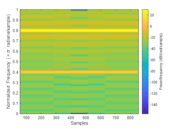
Use the waterplot function to plot the two outputs. Divide the frequency axis by π in both cases. For the stft output, divide the sample numbers by the effective sample rate, 2π.

figure nexttile waterplot(sx,fx/pi,tx) title("spectrogram")

nexttile waterplot(st,ft/pi,tt/(2*pi)) title("stft")

function waterplot(s,f,t) % Waterfall plot of spectrogram waterfall(f,t,abs(s)'.^2) set(gca,XDir="reverse",View=[30 50]) xlabel("Frequency/\pi") ylabel("Samples") end

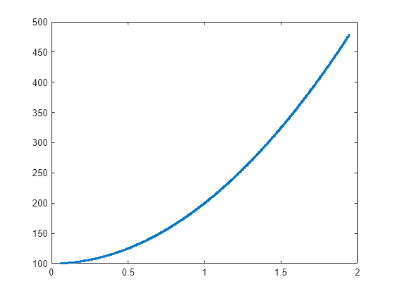
Use the spectrogram function to measure and track the instantaneous frequency of a signal.

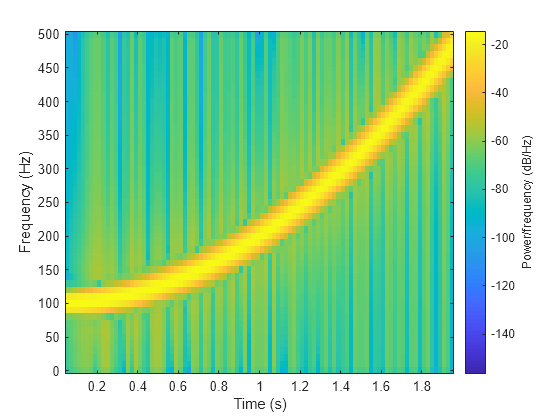
Generate a quadratic chirp sampled at 1 kHz for two seconds. Specify the chirp so that its frequency is initially 100 Hz and increases to 200 Hz after one second.

fs = 1000; t = 0:1/fs:2-1/fs; y = chirp(t,100,1,200,'quadratic');

Estimate the spectrum of the chirp using the short-time Fourier transform implemented in the spectrogram function. Divide the signal into sections of length 100, windowed with a Hamming window. Specify 80 samples of overlap between adjoining sections and evaluate the spectrum at ⌊100/2+1⌋=51 frequencies.

spectrogram(y,100,80,100,fs,'yaxis')

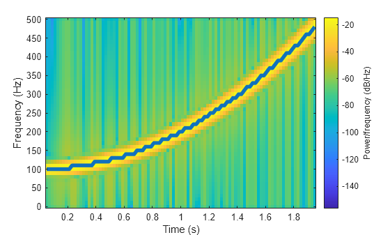
Track the chirp frequency by finding the time-frequency ridge with highest energy across the ⌊(2000-80)/(100-80)⌋=96 time points. Overlay the instantaneous frequency on the spectrogram plot.

[~,f,t,p] = spectrogram(y,100,80,100,fs);

[fridge,~,lr] = tfridge(p,f);

hold on plot3(t,fridge,abs(p(lr)),'LineWidth',4) hold off

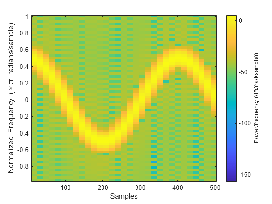
Generate 512 samples of a chirp with sinusoidally varying frequency content.

N = 512; n = 0:N-1;

x = exp(1jpisin(8*n/N)*32);

Compute the centered two-sided short-time Fourier transform of the chirp. Divide the signal into 32-sample segments with 16-sample overlap. Specify 64 DFT points. Plot the spectrogram.

[scalar,fs,ts] = spectrogram(x,32,16,64,'centered');

spectrogram(x,32,16,64,'centered','yaxis')

Obtain the same result by computing the spectrogram on 64 equispaced frequencies over the interval (-π,π]. The 'centered' option is not necessary.

fintv = -pi+pi/32:pi/32:pi;

[vector,fv,tv] = spectrogram(x,32,16,fintv);

spectrogram(x,32,16,fintv,'yaxis')

Generate a signal that consists of a voltage-controlled oscillator and three Gaussian atoms. The signal is sampled at fs=2 kHz for 2 seconds.

fs = 2000; tx = 0:1/fs:2; gaussFun = @(A,x,mu,f) exp(-(x-mu).^2/(20.03^2)).sin(2pif.*x)*A'; s = gaussFun([1 1 1],tx',[0.1 0.65 1],[2 6 2]*100)*1.5; x = vco(chirp(tx+.1,0,tx(end),3).exp(-2(tx-1).^2),[0.1 0.4]*fs,fs); x = s+x';

Short-Time Fourier Transforms

Use the pspectrum function to compute the STFT.

• Divide the Nx-sample signal into segments of length M=80 samples, corresponding to a time resolution of 80/2000=40 milliseconds.
• Specify L=16 samples or 20% of overlap between adjoining segments.
• Window each segment with a Kaiser window and specify a leakage ℓ=0.7.

M = 80; L = 16; lk = 0.7;

[S,F,T] = pspectrum(x,fs,"spectrogram", ... TimeResolution=M/fs,OverlapPercent=L/M*100, ... Leakage=lk);

Compare to the result obtained with the spectrogram function.

• Specify the window length and overlap directly in samples.
• pspectrum always uses a Kaiser window as g(n). The leakage ℓ and the shape factor β of the window are related by β=40×(1-ℓ).
• pspectrum always uses NDFT=1024 points when computing the discrete Fourier transform. You can specify this number if you want to compute the transform over a two-sided or centered frequency range. However, for one-sided transforms, which are the default for real signals, spectrogram uses 1024/2+1=513 points. Alternatively, you can specify the vector of frequencies at which you want to compute the transform, as in this example.
• If a signal cannot be divided exactly into k=⌊Nx-LM-L⌋ segments, spectrogram truncates the signal whereas pspectrum pads the signal with zeros to create an extra segment. To make the outputs equivalent, remove the final segment and the final element of the time vector.
• spectrogram returns the STFT, whose magnitude squared is the spectrogram. pspectrum returns the segment-by-segment power spectrum, which is already squared but is divided by a factor of ∑ng(n) before squaring.
• For one-sided transforms, pspectrum adds an extra factor of 2 to the spectrogram.

g = kaiser(M,40*(1-lk));

k = (length(x)-L)/(M-L); if k~=floor(k) S = S(:,1:floor(k)); T = T(1:floor(k)); end

[s,f,t] = spectrogram(x/sum(g)*sqrt(2),g,L,F,fs);

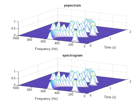
Use the waterplot function to display the spectrograms computed by the two functions.

subplot(2,1,1) waterplot(sqrt(S),F,T) title("pspectrum")

subplot(2,1,2) waterplot(s,f,t) title("spectrogram")

maxd = max(max(abs(abs(s).^2-S)))

Power Spectra and Convenience Plots

The spectrogram function has a fourth argument that corresponds to the segment-by-segment power spectrum or power spectral density. Similar to the output of pspectrum, the ps argument is already squared and includes the normalization factor ∑ng(n). For one-sided spectrograms of real signals, you still have to include the extra factor of 2. Set the scaling argument of the function to "power".

[,,~,ps] = spectrogram(x*sqrt(2),g,L,F,fs,"power");

max(abs(S(:)-ps(:)))

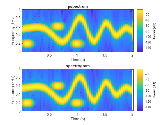
When called with no output arguments, both pspectrum and spectrogram plot the spectrogram of the signal in decibels. Include the factor of 2 for one-sided spectrograms. Set the colormaps to be the same for both plots. Set the _x_-limits to the same values to make visible the extra segment at the end of the pspectrum plot. In the spectrogram plot, display the frequency on the _y_-axis.

subplot(2,1,1) pspectrum(x,fs,"spectrogram", ... TimeResolution=M/fs,OverlapPercent=L/M*100, ... Leakage=lk) title("pspectrum") cc = clim; xl = xlim;

subplot(2,1,2) spectrogram(x*sqrt(2),g,L,F,fs,"power","yaxis") title("spectrogram") clim(cc) xlim(xl)

function waterplot(s,f,t) % Waterfall plot of spectrogram waterfall(f,t,abs(s)'.^2) set(gca,XDir="reverse",View=[30 50]) xlabel("Frequency (Hz)") ylabel("Time (s)") end

Generate a chirp signal sampled for 2 seconds at 1 kHz. Specify the chirp so that its frequency is initially 100 Hz and increases to 200 Hz after 1 second.

fs = 1000; t = 0:1/fs:2; y = chirp(t,100,1,200,"quadratic");

Estimate the reassigned spectrogram of the signal.

• Divide the signal into sections of length 128, windowed with a Kaiser window with shape parameter β=18.
• Specify 120 samples of overlap between adjoining sections.
• Evaluate the spectrum at ⌊128/2⌋=65 frequencies and ⌊(length(x)-120)/(128-120)⌋=235 time bins.

Use the spectrogram function with no output arguments to plot the reassigned spectrogram. Display frequency on the _y_-axis and time on the _x_-axis.

spectrogram(y,kaiser(128,18),120,128,fs, ... "reassigned","yaxis")

Redo the plot using the imagesc function. Specify the _y_-axis direction so that the frequency values increase from bottom to top. Add eps to the reassigned spectrogram to avoid potential negative infinities when converting to decibels.

[~,fr,tr,pxx] = spectrogram(y,kaiser(128,18),120,128,fs, ... "reassigned");

imagesc(tr,fr,pow2db(pxx+eps)) axis xy xlabel("Time (s)") ylabel("Frequency (Hz)") colorbar

Generate a chirp signal sampled for 2 seconds at 1 kHz. Specify the chirp so that its frequency is initially 100 Hz and increases to 200 Hz after 1 second.

Fs = 1000; t = 0:1/Fs:2; y = chirp(t,100,1,200,'quadratic');

Estimate the time-dependent power spectral density (PSD) of the signal.

• Divide the signal into sections of length 128, windowed with a Kaiser window with shape parameter β=18.
• Specify 120 samples of overlap between adjoining sections.
• Evaluate the spectrum at ⌊128/2⌋=65 frequencies and ⌊(length(x)-120)/(128-120)⌋=235 time bins.

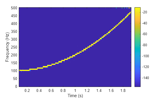
Output the frequency and time of the center of gravity of each PSD estimate. Set to zero those elements of the PSD smaller than -30 dB.

[,,~,pxx,fc,tc] = spectrogram(y,kaiser(128,18),120,128,Fs, ... 'MinThreshold',-30);

Plot the nonzero elements as functions of the center-of-gravity frequencies and times.

plot(tc(pxx>0),fc(pxx>0),'.')

Generate a signal that consists of a real-valued chirp sampled at 2 kHz for 2 seconds.

fs = 2000; tx = 0:1/fs:2; x = vco(-chirp(tx,0,tx(end),2).exp(-3(tx-1).^2), ... [0.1 0.4]*fs,fs).*hann(length(tx))';

Two-Sided Spectrogram

Compute and plot the two-sided STFT of the signal.

• Divide the signal into segments, each M=73 samples long.
• Specify L=24 samples of overlap between adjoining segments.
• Discard the final, shorter segment.
• Window each segment with a flat-top window.
• Evaluate the discrete Fourier transform of each segment at NDFT=895 points, noting that it is an odd number.

M = 73; L = 24; g = flattopwin(M); Ndft = 895; neven = ~mod(Ndft,2);

[stwo,f,t] = spectrogram(x,g,L,Ndft,fs,"twosided");

Use the spectrogram function with no output arguments to plot the two-sided spectrogram.

spectrogram(x,g,L,Ndft,fs,"twosided","power","yaxis")

Compute the two-sided spectrogram using the definition. Divide the signal into M-sample segments with L samples of overlap between adjoining segments. Window each segment and compute its discrete Fourier transform at NDFT points.

y = framesig(x,M,Window=g,OverlapLength=L); Xtwo = fft(y,Ndft);

Compute the time and frequency ranges.

• To find the time values, divide the time vector into overlapping segments. The time values are the midpoints of the segments, with each segment treated as an interval open at the lower end.
• To find the frequency values, specify a Nyquist interval closed at zero frequency and open at the upper end.

framedT = framesig(tx,M,OverlapLength=L); ttwo = mean(framedT(2:end,:));

ftwo = 0:fs/Ndft:fs*(1-1/Ndft);

Compare the outputs of spectrogram to the definitions. Use the waterplot function to display the spectrograms.

diffs = [max(max(abs(stwo-Xtwo))); max(abs(f-ftwo')); max(abs(t-ttwo))]

diffs = 3×1 10-12 ×

     0
0.2274
0.0002

figure nexttile waterplot(Xtwo,ftwo,ttwo) title("Two-Sided, Definition")

nexttile waterplot(stwo,f,t) title("Two-Sided, spectrogram Function")

Centered Spectrogram

Compute the centered spectrogram of the signal.

• Use the same time values that you used for the two-sided STFT.
• Use the fftshift function to shift the zero-frequency component of the STFT to the center of the spectrum.
• For odd-valued NDFT, the frequency interval is open at both ends. For even-valued NDFT, the frequency interval is open at the lower end and closed at the upper end.

Compare the outputs and display the spectrograms.

tcen = ttwo;

if ~neven Xcen = fftshift(Xtwo,1); fcen = -fs/2*(1-1/Ndft):fs/Ndft:fs/2; else Xcen = fftshift(circshift(Xtwo,-1),1); fcen = (-fs/2*(1-1/Ndft):fs/Ndft:fs/2)+fs/Ndft/2; end

[scen,f,t] = spectrogram(x,g,L,Ndft,fs,"centered");

diffs = [max(max(abs(scen-Xcen))); max(abs(f-fcen')); max(abs(t-tcen))]

diffs = 3×1 10-12 ×

     0
0.2274
0.0002

figure nexttile waterplot(Xcen,fcen,tcen) title("Centered, Definition")

nexttile waterplot(scen,f,t) title("Centered, spectrogram Function")

One-Sided Spectrogram

Compute the one-sided spectrogram of the signal.

• Use the same time values that you used for the two-sided STFT.
• For odd-valued NDFT, the one-sided STFT consists of the first (NDFT+1)/2 rows of the two-sided STFT. For even-valued NDFT, the one-sided STFT consists of the first NDFT/2+1 rows of the two-sided STFT.
• For odd-valued NDFT, the frequency interval is closed at zero frequency and open at the Nyquist frequency. For even-valued NDFT, the frequency interval is closed at both ends.

Compare the outputs and display the spectrograms. For real-valued signals, the "onesided" argument is optional.

tone = ttwo;

if ~neven Xone = Xtwo(1:(Ndft+1)/2,:); else Xone = Xtwo(1:Ndft/2+1,:); end

fone = 0:fs/Ndft:fs/2;

[sone,f,t] = spectrogram(x,g,L,Ndft,fs);

diffs = [max(max(abs(sone-Xone))); max(abs(f-fone')); max(abs(t-tone))]

diffs = 3×1 10-12 ×

     0
0.1137
0.0002

figure nexttile waterplot(Xone,fone,tone) title("One-Sided, Definition")

nexttile waterplot(sone,f,t) title("One-Sided, spectrogram Function")

function waterplot(s,f,t) % Waterfall plot of spectrogram waterfall(f,t,abs(s)'.^2) set(gca,XDir="reverse",View=[30 50]) xlabel("Frequency (Hz)") ylabel("Time (s)") end

The spectrogram function has a matrix containing either the power spectral density (PSD) or the power spectrum of each segment as the fourth output argument. The power spectrum is equal to the PSD multiplied by the equivalent noise bandwidth (ENBW) of the window.

Generate a signal that consists of a logarithmic chirp sampled at 1 kHz for 1 second. The chirp has an initial frequency of 400 Hz that decreases to 10 Hz by the end of the measurement.

fs = 1000; tt = 0:1/fs:1-1/fs; y = chirp(tt,400,tt(end),10,"logarithmic");

Segment PSDs and Power Spectra with Sample Rate

Divide the signal into 102-sample segments and window each segment with a Hann window. Specify 12 samples of overlap between adjoining segments and 1024 DFT points.

M = 102; g = hann(M); L = 12; Ndft = 1024;

Compute the spectrogram of the signal with the default PSD spectrum type. Output the STFT and the array of segment power spectral densities.

[s,f,t,p] = spectrogram(y,g,L,Ndft,fs);

Repeat the computation with the spectrum type specified as "power". Output the STFT and the array of segment power spectra.

[r,,,q] = spectrogram(y,g,L,Ndft,fs,"power");

Verify that the spectrogram is the same in both cases. Plot the spectrogram using a logarithmic scale for the frequency.

max(max(abs(s).^2-abs(r).^2))

waterfall(f,t,abs(s)'.^2) set(gca,XScale="log",... XDir="reverse",View=[30 50])

Verify that the power spectra are equal to the power spectral densities multiplied by the ENBW of the window.

max(max(abs(q-p*enbw(g,fs))))

Verify that the matrix of segment power spectra is proportional to the spectrogram. The proportionality factor is the square of the sum of the window elements.

max(max(abs(s).^2-q*sum(g)^2))

Segment PSDs and Power Spectra with Normalized Frequencies

Repeat the computation, but now work in normalized frequencies. The results are the same when you specify the sample rate as 2π.

[,,,pn] = spectrogram(y,g,L,Ndft); [,,,qn] = spectrogram(y,g,L,Ndft,"power");

max(max(abs(qn-pnenbw(g,2pi))))

Load an audio signal that contains two decreasing chirps and a wideband splatter sound. Compute the short-time Fourier transform. Divide the waveform into 400-sample segments with 300-sample overlap. Plot the spectrogram.

load splat

% To hear, type soundsc(y,Fs)

sg = 400; ov = 300;

spectrogram(y,sg,ov,[],Fs,"yaxis") colormap bone

Use the spectrogram function to output the power spectral density (PSD) of the signal.

[s,f,t,p] = spectrogram(y,sg,ov,[],Fs);

Track the two chirps using the medfreq function. To find the stronger, low-frequency chirp, restrict the search to frequencies above 100 Hz and to times before the start of the wideband sound.

f1 = f > 100; t1 = t < 0.75;

m1 = medfreq(p(f1,t1),f(f1));

To find the faint high-frequency chirp, restrict the search to frequencies above 2500 Hz and to times between 0.3 seconds and 0.65 seconds.

f2 = f > 2500; t2 = t > 0.3 & t < 0.65;

m2 = medfreq(p(f2,t2),f(f2));

Overlay the result on the spectrogram. Divide the frequency values by 1000 to express them in kHz.

hold on plot(t(t1),m1/1000,LineWidth=4) plot(t(t2),m2/1000,LineWidth=4) hold off

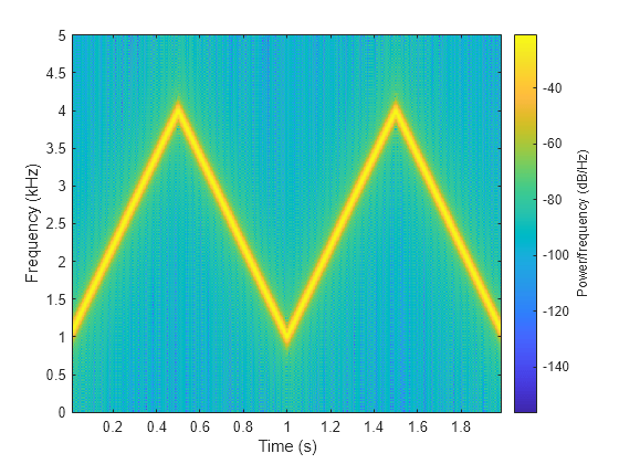
Generate two seconds of a signal sampled at 10 kHz. Specify the instantaneous frequency of the signal as a triangular function of time.

fs = 10e3; t = 0:1/fs:2; x1 = vco(sawtooth(2pit,0.5),[0.1 0.4]*fs,fs);

Compute and plot the spectrogram of the signal. Use a Kaiser window of length 256 and shape parameter β=5. Specify 220 samples of section-to-section overlap and 512 DFT points. Plot the frequency on the _y_-axis. Use the default colormap and view.

spectrogram(x1,kaiser(256,5),220,512,fs,'yaxis')

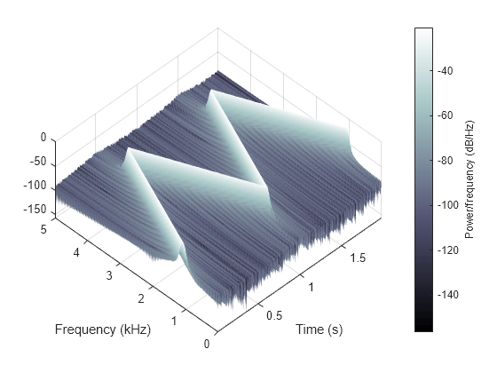
Change the view to display the spectrogram as a waterfall plot. Set the colormap to bone.

view(-45,65) colormap bone

Since R2025a

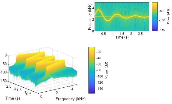
Plot the spectrograms for four signals in axes handles and panel containers. When you use spectrogram without output arguments, the function returns a convenience plot with the power spectral density (PSD) estimate. To reproduce this plot on a specific axes handle or panel container, specify spectrogram with a target Parent input argument.

Create four oscillating signals with a sample rate of 10 kHz for three seconds.

• x1: Sawtooth-shaped oscillating signal
• x2: Exponentially decaying oscillating signal
• x3: Complex sinusoidal envelope
• x4: Quadratic-sweeping chirp

Fs = 10e3; t = 0:1/Fs:3; x1 = vco(sawtooth(2pit,0.5),[0.1 0.4]Fs,Fs); x2 = vco(sin(2pit).exp(-t),[0.1 0.4]Fs,Fs) ... + 0.01sin(2pi0.25Fst); x3 = exp(1jpisin(4*t)*Fs/10); x4 = chirp(t,Fs/10,t(end),Fs/2.5,"quadratic");

Define specifications to calculate the signal spectrograms: 512 DFT points, a 256-sample Kaiser window, and an overlap length of 220 samples.

nfft = 512; g = kaiser(256,5); ol = 220;

Plot Spectrograms in Axes Handle

Create two axes handles in the southwestern and northeastern corners of a new figure window.

fig = figure; ax1 = axes(fig,Position=[0.05 0.1 0.55 0.45]); ax2 = axes(fig,Position=[0.55 0.7 0.42 0.28]);

Plot the power spectra of the signals x1 and x2 in the southwestern and northeastern axes of the figure, respectively. View the spectrogram of x1 in the default 3-D line of sight. Display the frequencies in the _y_-axis for the spectrogram of x2.

spectrogram(x1,g,ol,nfft,Fs,"power",Parent=ax1); view(ax1,3); spectrogram(x2,g,ol,nfft,Fs,"power","yaxis",Parent=ax2);

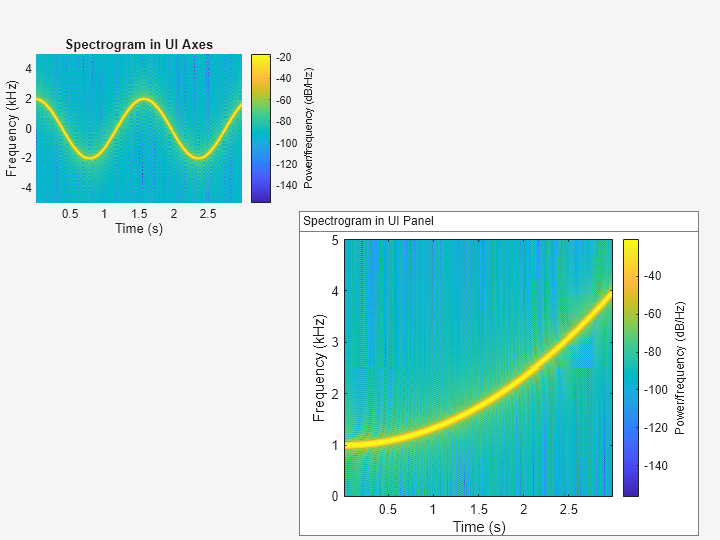
Plot Spectrogram in UI-based Axes Handle

Create an axes handle in the northwestern corner of a new UI figure window.

uif = uifigure(Position=[100 100 720 540]); ax3 = uiaxes(uif,'Position',[5 305 300 200]);

Plot the PSD estimate of the signal x3 on the figure axes. Display the frequencies in the _y_-axis and centered in 0 kHz.

spectrogram(x3,g,ol,nfft,Fs,"centered","yaxis",Parent=ax3); title(ax3,"Spectrogram in UI Axes")

Plot Spectrogram in Panel Container

Add a panel container in the southeastern corner of the UI figure window.

ax4 = uipanel(uif,Position=[300 5 400 325], ... Title="Spectrogram in UI Panel", ... BackgroundColor="white");

Plot the PSD estimate of the signal x4 on the panel container. Display the frequencies in the _y_-axis.

spectrogram(x4,g,ol,nfft,Fs,"yaxis",Parent=ax4);

Input Arguments

collapse all

Input signal, specified as a row or column vector.

Example: cos(pi/4*(0:159))+randn(1,160) specifies a sinusoid embedded in white Gaussian noise.

Data Types: single | double
Complex Number Support: Yes

Window, specified as a positive integer or as a row or column vector. Usewindow to divide the signal into segments:

• If window is an integer, thenspectrogram dividesx into segments of lengthwindow and windows each segment with a Hamming window of that length.
• If window is a vector, thenspectrogram dividesx into segments of the same length as the vector and windows each segment usingwindow.

If the length of x cannot be divided exactly into an integer number of segments withnoverlap overlapping samples, thenx is truncated accordingly.

If you specify window as empty, thenspectrogram uses a Hamming window such thatx is divided into eight segments withnoverlap overlapping samples.

For a list of available windows, see Windows.

Example: hann(N+1) and(1-cos(2*pi*(0:N)'/N))/2 both specify a Hann window of length N + 1.

Number of overlapped samples, specified as a nonnegative integer.

• If window is scalar, thennoverlap must be smaller thanwindow.
• If window is a vector, thennoverlap must be smaller than the length of window.

If you specify noverlap as empty, thenspectrogram uses a number that produces 50% overlap between segments. If the segment length is unspecified, the function setsnoverlap to ⌊Nx/4.5⌋, where Nx is the length of the input signal and the ⌊⌋ symbols denote the floor function.

Number of DFT points, specified as a positive integer scalar. If you specify nfft as empty, thenspectrogram sets the parameter to max(256,2_p_), where p = ⌈log2 _Nw_⌉, the ⌈⌉ symbols denote the ceiling function, and

• Nw =window if window is a scalar.
• Nw =length(`window`) if window is a vector.

Normalized frequencies, specified as a vector. w must have at least two elements, because otherwise the function interprets it asnfft. Normalized frequencies are in rad/sample.

Example: pi./[2 4]

Data Types: single | double

Cyclical frequencies, specified as a vector. f must have at least two elements, because otherwise the function interprets it asnfft. The units of f are specified by the sample rate, fs.

Data Types: single | double

Sample rate, specified as a positive scalar. The sample rate is the number of samples per unit time. If the unit of time is seconds, then the sample rate is in Hz.

Frequency range for the PSD estimate, specified as"onesided", "twosided", or"centered". For real-valued signals, the default is"onesided". For complex-valued signals, the default is "twosided", and specifying"onesided" results in an error.

• "onesided" — returns the one-sided spectrogram of a real input signal. If nfft is even, then ps has nfft/2 + 1 rows and is computed over the interval [0, _π_] rad/sample. If nfft is odd, then ps has (nfft + 1)/2 rows and the interval is [0, _π_) rad/sample. If you specifyfs, then the intervals are respectively [0,fs/2] cycles/unit time and [0,fs/2) cycles/unit time.
• "twosided" — returns the two-sided spectrogram of a real or complex-valued signal.ps has nfft rows and is computed over the interval [0, 2_π_) rad/sample. If you specifyfs, then the interval is [0,fs) cycles/unit time.
• "centered" — returns the centered two-sided spectrogram of a real or complex-valued signal.ps has nfft rows. Ifnfft is even, then ps is computed over the interval (–π,π_] rad/sample. If nfft is odd, then ps is computed over (–_π,π) rad/sample. If you specifyfs, then the intervals are respectively (–fs/2, fs/2] cycles/unit time and (–fs/2,fs/2) cycles/unit time.

Data Types: char | string

Power spectrum scaling, specified as "psd" or"power".

• Omitting spectrumtype, or specifying"psd", returns the power spectral density.
• Specifying "power" scales each estimate of the PSD by the equivalent noise bandwidth of the window. The result is an estimate of the power at each frequency. If the"reassigned" option is on, the function integrates the PSD over the width of each frequency bin before reassigning.

Data Types: char | string

Frequency display axis, specified as "xaxis" or"yaxis".

• "xaxis" — displays frequency on the_x_-axis and time on the_y_-axis.
• "yaxis" — displays frequency on the_y_-axis and time on the_x_-axis.

This argument is ignored if you callspectrogram with output arguments.

Data Types: char | string

Name-Value Arguments

collapse all

Specify optional pairs of arguments asName1=Value1,...,NameN=ValueN, where Name is the argument name and Value is the corresponding value. Name-value arguments must appear after other arguments, but the order of the pairs does not matter.

Example: spectrogram(x,100,OutputTimeDimension="downrows") divides x into segments of length 100 and windows each segment with a Hamming window of that length The output of the spectrogram has time dimension down the rows.

Before R2021a, use commas to separate each name and value, and enclose Name in quotes.

Example: spectrogram(x,100,'OutputTimeDimension','downrows') divides x into segments of length 100 and windows each segment with a Hamming window of that length The output of the spectrogram has time dimension down the rows.

Threshold, specified as a real scalar expressed in decibels.spectrogram sets to zero those elements ofs such that 10 log10(s) ≤ thresh.

Output time dimension, specified as "acrosscolumns" or "downrows". Set this value to"downrows", if you want the time dimension ofs, ps,fc, and tc down the rows and the frequency dimension along the columns. Set this value to"acrosscolumns", if you want the time dimension of s, ps,fc, and tc across the columns and frequency dimension along the rows. This input is ignored if the function is called without output arguments.

Data Types: char | string

Since R2025a

Target parent, specified as an Axes object, UIAxes object, or Panel object.

• If you specify Parent, thespectrogram function plots the PSD or power spectrum as a surface plot on the specified target parent. The function returns the plot even if you call it with or without output arguments.
• If you do not specify Parent and you do not specify output arguments, thespectrogram function plots the PSD or power spectrum as a surface plot on the current axes or chart that gca returns.

For more information about targets, see Graphics Objects. For more information about the parent-child relationship in MATLAB® graphics, see Graphics Object Hierarchy.

Data Types: Axes | UIAxes | Panel

Output Arguments

collapse all

Short-time Fourier transform, returned as a matrix. Time increases across the columns of s and frequency increases down the rows, starting from zero.

• If x is a signal of length_Nx_, thens has k columns, where
  • k = ⌊(Nx –noverlap)/(window – noverlap)⌋ ifwindow is a scalar.
  • k = ⌊(Nx –noverlap)/(length(`window`) – noverlap)⌋ ifwindow is a vector.
• If x is real andnfft is even, thens has (nfft/2 + 1) rows.
• If x is real andnfft is odd, thens has (nfft + 1)/2 rows.
• If x is complex-valued, thens has nfft rows.

Note

When freqrange is set to"onesided", spectrogram outputs the s values in the positive Nyquist range and does not conserve the total power.

s is not affected by the"reassigned" option.

Normalized frequencies, returned as a vector. w has a length equal to the number of rows of s.

Time instants, returned as a vector. The time values int correspond to the midpoint of each segment.

Cyclical frequencies, returned as a vector. f has a length equal to the number of rows of s.

Power spectral density (PSD) or power spectrum, returned as a matrix.

• If x is real andfreqrange is left unspecified or set to"onesided", then ps contains the one-sided modified periodogram estimate of the PSD or power spectrum of each segment. The function multiplies the power by 2 at all frequencies except 0 and the Nyquist frequency to conserve the total power.
• If x is complex-valued or iffreqrange is set to"twosided" or"centered", then ps contains the two-sided modified periodogram estimate of the PSD or power spectrum of each segment.
• If you specify a vector of normalized frequencies in w or a vector of cyclical frequencies in f, thenps contains the modified periodogram estimate of the PSD or power spectrum of each segment evaluated at the input frequencies.

Center-of-energy frequencies and times, returned as matrices of the same size as the short-time Fourier transform. If you do not specify a sample rate, then the elements of fc are returned as normalized frequencies.

More About

collapse all

The short-time Fourier transform (STFT) is used to analyze how the frequency content of a nonstationary signal changes over time. The magnitude squared of the STFT is known as the spectrogram time-frequency representation of the signal. For more information about the spectrogram and how to compute it using Signal Processing Toolbox™ functions, see Spectrogram Computation with Signal Processing Toolbox.

The STFT of a signal is computed by sliding an analysis window g(n) of length M over the signal and calculating the discrete Fourier transform (DFT) of each segment of windowed data. The window hops over the original signal at intervals of R samples, equivalent to L = M –R samples of overlap between adjoining segments. Most window functions taper off at the edges to avoid spectral ringing. The DFT of each windowed segment is added to a complex-valued matrix that contains the magnitude and phase for each point in time and frequency. The STFT matrix has

columns, where Nx is the length of the signal x(n) and the ⌊⌋ symbols denote the floor function. The number of rows in the matrix equals _N_DFT, the number of DFT points, for centered and two-sided transforms and an odd number close to _N_DFT/2 for one-sided transforms of real-valued signals.

The _m_th column of the STFT matrix X(f)=[X1(f)X2(f)X3(f)⋯Xk(f)] contains the DFT of the windowed data centered about time mR:

Tips

If a short-time Fourier transform has zeros, its conversion to decibels results in negative infinities that cannot be plotted. To avoid this potential difficulty, spectrogram adds eps to the short-time Fourier transform when you call it with no output arguments.

References

[1] Boashash, Boualem, ed.Time Frequency Signal Analysis and Processing: A Comprehensive Reference. Second edition. EURASIP and Academic Press Series in Signal and Image Processing. Amsterdam and Boston: Academic Press, 2016.

[2] Chassande-Motin, Éric, François Auger, and Patrick Flandrin. "Reassignment." In Time-Frequency Analysis: Concepts and Methods. Edited by Franz Hlawatsch and François Auger. London: ISTE/John Wiley and Sons, 2008.

[3] Fulop, Sean A., and Kelly Fitz. "Algorithms for computing the time-corrected instantaneous frequency (reassigned) spectrogram, with applications." Journal of the Acoustical Society of America. Vol. 119, January 2006, pp. 360–371.

[4] Oppenheim, Alan V., and Ronald W. Schafer, with John R. Buck. Discrete-Time Signal Processing. Second edition. Upper Saddle River, NJ: Prentice Hall, 1999.

[5] Rabiner, Lawrence R., and Ronald W. Schafer. Digital Processing of Speech Signals. Englewood Cliffs, NJ: Prentice-Hall, 1978.

Extended Capabilities

expand all

Thespectrogram function supports tall arrays with the following usage notes and limitations:

• Input must be a tall column vector.
• The window argument must always be specified.
• OutputTimeDimension must be always specified and set to "downrows".
• The reassigned option is not supported.
• Syntaxes with no output arguments are not supported.

For more information, see Tall Arrays.

Usage notes and limitations:

• The Parent input argument is not supported.
• Arguments specified using name-value arguments must be compile-time constants.

Usage notes and limitations:

• Arguments specified using name-value arguments must be compile-time constants.
• Variable-size window must be double precision.

Version History

Introduced before R2006a

expand all

The spectrogram function supports plotting the power spectrum density (PSD) estimate or power spectrum in one of these target-parent objects:Axes, UIAxes, or Panel.

The spectrogram function supports single-precision variable-size window inputs for code generation.

The spectrogram function supports single-precision inputs and code generation for graphical processing units (GPUs). You must have MATLAB Coder™ and GPU Coder™ to generate CUDA® code.

You can now use the Create Plot Live Editor task to visualize the output ofspectrogram interactively. You can select different chart types and set optional parameters. The task also automatically generates code that becomes part of your live script.

See Also

Apps

• Signal Analyzer

Functions

• goertzel | istft | periodogram | pspectrum | pwelch | stft | xspectrogram

Topics

• Spectrogram Computation with Signal Processing Toolbox
• Time-Frequency Gallery
• Practical Introduction to Time-Frequency Analysis
• Formant Estimation with LPC Coefficients