Working with missing data — pandas 3.0.1 documentation (original) (raw)
Values considered “missing”#
pandas uses different sentinel values to represent a missing (also referred to as NA) depending on the data type.
numpy.nan for NumPy data types. The disadvantage of using NumPy data types is that the original data type will be coerced to np.float64 or object.
In [1]: pd.Series([1, 2], dtype=np.int64).reindex([0, 1, 2]) Out[1]: 0 1.0 1 2.0 2 NaN dtype: float64
In [2]: pd.Series([True, False], dtype=np.bool_).reindex([0, 1, 2]) Out[2]: 0 True 1 False 2 NaN dtype: object
NaT for NumPy np.datetime64, np.timedelta64, and PeriodDtype. For typing applications, use api.typing.NaTType.
In [3]: pd.Series([1, 2], dtype=np.dtype("timedelta64[ns]")).reindex([0, 1, 2]) Out[3]: 0 0 days 00:00:00.000000001 1 0 days 00:00:00.000000002 2 NaT dtype: timedelta64[ns]
In [4]: pd.Series([1, 2], dtype=np.dtype("datetime64[ns]")).reindex([0, 1, 2]) Out[4]: 0 1970-01-01 00:00:00.000000001 1 1970-01-01 00:00:00.000000002 2 NaT dtype: datetime64[ns]
In [5]: pd.Series(["2020", "2020"], dtype=pd.PeriodDtype("D")).reindex([0, 1, 2]) Out[5]: 0 2020-01-01 1 2020-01-01 2 NaT dtype: period[D]
NA for StringDtype, Int64Dtype (and other bit widths),Float64Dtype (and other bit widths), BooleanDtype and ArrowDtype. These types will maintain the original data type of the data. For typing applications, use api.typing.NAType.
In [6]: pd.Series([1, 2], dtype="Int64").reindex([0, 1, 2]) Out[6]: 0 1 1 2 2 dtype: Int64
In [7]: pd.Series([True, False], dtype="boolean[pyarrow]").reindex([0, 1, 2]) Out[7]: 0 True 1 False 2 dtype: bool[pyarrow]
To detect these missing value, use the isna() or notna() methods.
In [8]: ser = pd.Series([pd.Timestamp("2020-01-01"), pd.NaT])
In [9]: ser Out[9]: 0 2020-01-01 1 NaT dtype: datetime64[us]
In [10]: pd.isna(ser) Out[10]: 0 False 1 True dtype: bool
Note
isna() or notna() will also consider None a missing value.
In [11]: ser = pd.Series([1, None], dtype=object)
In [12]: ser Out[12]: 0 1 1 None dtype: object
In [13]: pd.isna(ser) Out[13]: 0 False 1 True dtype: bool
Warning
Equality comparisons between np.nan, NaT, and NAdo not act like None
In [14]: None == None # noqa: E711 Out[14]: True
In [15]: np.nan == np.nan Out[15]: False
In [16]: pd.NaT == pd.NaT Out[16]: False
In [17]: pd.NA == pd.NA Out[17]:
Therefore, an equality comparison between a DataFrame or Serieswith one of these missing values does not provide the same information asisna() or notna().
In [18]: ser = pd.Series([True, None], dtype="boolean[pyarrow]")
In [19]: ser == pd.NA Out[19]: 0 1 dtype: bool[pyarrow]
In [20]: pd.isna(ser) Out[20]: 0 False 1 True dtype: bool
NA semantics#
Warning
Experimental: the behaviour of NA can still change without warning.
Starting from pandas 1.0, an experimental NA value (singleton) is available to represent scalar missing values. The goal of NA is provide a “missing” indicator that can be used consistently across data types (instead of np.nan, None or pd.NaT depending on the data type).
For example, when having missing values in a Series with the nullable integer dtype, it will use NA:
In [21]: s = pd.Series([1, 2, None], dtype="Int64")
In [22]: s Out[22]: 0 1 1 2 2 dtype: Int64
In [23]: s[2] Out[23]:
In [24]: s[2] is pd.NA Out[24]: True
Currently, pandas does not use those data types using NA by default in a DataFrame or Series, so you need to specify the dtype explicitly. An easy way to convert to those dtypes is explained in theconversion section.
Propagation in arithmetic and comparison operations#
In general, missing values propagate in operations involving NA. When one of the operands is unknown, the outcome of the operation is also unknown.
For example, NA propagates in arithmetic operations, similarly tonp.nan:
In [25]: pd.NA + 1 Out[25]:
In [26]: "a" * pd.NA Out[26]:
There are a few special cases when the result is known, even when one of the operands is NA.
In [27]: pd.NA ** 0 Out[27]: 1
In [28]: 1 ** pd.NA Out[28]: 1
In equality and comparison operations, NA also propagates. This deviates from the behaviour of np.nan, where comparisons with np.nan always return False.
In [29]: pd.NA == 1 Out[29]:
In [30]: pd.NA == pd.NA Out[30]:
In [31]: pd.NA < 2.5 Out[31]:
To check if a value is equal to NA, use isna()
In [32]: pd.isna(pd.NA) Out[32]: True
Note
An exception on this basic propagation rule are reductions (such as the mean or the minimum), where pandas defaults to skipping missing values. See thecalculation section for more.
Logical operations#
For logical operations, NA follows the rules of thethree-valued logic (or_Kleene logic_, similarly to R, SQL and Julia). This logic means to only propagate missing values when it is logically required.
For example, for the logical “or” operation (|), if one of the operands is True, we already know the result will be True, regardless of the other value (so regardless the missing value would be True or False). In this case, NA does not propagate:
In [33]: True | False Out[33]: True
In [34]: True | pd.NA Out[34]: True
In [35]: pd.NA | True Out[35]: True
On the other hand, if one of the operands is False, the result depends on the value of the other operand. Therefore, in this case NApropagates:
In [36]: False | True Out[36]: True
In [37]: False | False Out[37]: False
In [38]: False | pd.NA Out[38]:
The behaviour of the logical “and” operation (&) can be derived using similar logic (where now NA will not propagate if one of the operands is already False):
In [39]: False & True Out[39]: False
In [40]: False & False Out[40]: False
In [41]: False & pd.NA Out[41]: False
In [42]: True & True Out[42]: True
In [43]: True & False Out[43]: False
In [44]: True & pd.NA Out[44]:
NA in a boolean context#
Since the actual value of an NA is unknown, it is ambiguous to convert NA to a boolean value.
In [45]: bool(pd.NA)
TypeError Traceback (most recent call last) Cell In[45], line 1 ----> 1 bool(pd.NA)
File ~/work/pandas/pandas/pandas/_libs/missing.pyx:415, in pandas._libs.missing.NAType.bool()
TypeError: boolean value of NA is ambiguous
This also means that NA cannot be used in a context where it is evaluated to a boolean, such as if condition: ... where condition can potentially be NA. In such cases, isna() can be used to check for NA or condition being NA can be avoided, for example by filling missing values beforehand.
A similar situation occurs when using Series or DataFrame objects in ifstatements, see Using if/truth statements with pandas.
NumPy ufuncs#
pandas.NA implements NumPy’s __array_ufunc__ protocol. Most ufuncs work with NA, and generally return NA:
In [46]: np.log(pd.NA) Out[46]:
In [47]: np.add(pd.NA, 1) Out[47]:
Warning
Currently, ufuncs involving an ndarray and NA will return an object-dtype filled with NA values.
In [48]: a = np.array([1, 2, 3])
In [49]: np.greater(a, pd.NA) Out[49]: array([, , ], dtype=object)
The return type here may change to return a different array type in the future.
See DataFrame interoperability with NumPy functions for more on ufuncs.
Conversion#
If you have a DataFrame or Series using np.nan,DataFrame.convert_dtypes() and Series.convert_dtypes(), respectively, will convert your data to use the nullable data types supporting NA, such as Int64Dtype or ArrowDtype. This is especially helpful after reading in data sets from IO methods where data types were inferred.
In [50]: import io
In [51]: data = io.StringIO("a,b\n,True\n2,")
In [52]: df = pd.read_csv(data)
In [53]: df.dtypes Out[53]: a float64 b object dtype: object
In [54]: df_conv = df.convert_dtypes()
In [55]: df_conv Out[55]: a b 0 True 1 2
In [56]: df_conv.dtypes Out[56]: a Int64 b boolean dtype: object
Inserting missing data#
You can insert missing values by simply assigning to a Series or DataFrame. The missing value sentinel used will be chosen based on the dtype.
In [57]: ser = pd.Series([1., 2., 3.])
In [58]: ser.loc[0] = None
In [59]: ser Out[59]: 0 NaN 1 2.0 2 3.0 dtype: float64
In [60]: ser = pd.Series([pd.Timestamp("2021"), pd.Timestamp("2021")])
In [61]: ser.iloc[0] = np.nan
In [62]: ser Out[62]: 0 NaT 1 2021-01-01 dtype: datetime64[us]
In [63]: ser = pd.Series([True, False], dtype="boolean[pyarrow]")
In [64]: ser.iloc[0] = None
In [65]: ser Out[65]: 0 1 False dtype: bool[pyarrow]
For object types, pandas will use the value given:
In [66]: s = pd.Series(["a", "b", "c"], dtype=object)
In [67]: s.loc[0] = None
In [68]: s.loc[1] = np.nan
In [69]: s Out[69]: 0 None 1 NaN 2 c dtype: object
Calculations with missing data#
Missing values propagate through arithmetic operations between pandas objects.
In [70]: ser1 = pd.Series([np.nan, np.nan, 2, 3])
In [71]: ser2 = pd.Series([np.nan, 1, np.nan, 4])
In [72]: ser1 Out[72]: 0 NaN 1 NaN 2 2.0 3 3.0 dtype: float64
In [73]: ser2 Out[73]: 0 NaN 1 1.0 2 NaN 3 4.0 dtype: float64
In [74]: ser1 + ser2 Out[74]: 0 NaN 1 NaN 2 NaN 3 7.0 dtype: float64
The descriptive statistics and computational methods discussed in thedata structure overview (and listed here and here) all account for missing data.
When summing data, NA values or empty data will be treated as zero.
In [75]: pd.Series([np.nan]).sum() Out[75]: np.float64(0.0)
In [76]: pd.Series([], dtype="float64").sum() Out[76]: np.float64(0.0)
When taking the product, NA values or empty data will be treated as 1.
In [77]: pd.Series([np.nan]).prod() Out[77]: np.float64(1.0)
In [78]: pd.Series([], dtype="float64").prod() Out[78]: np.float64(1.0)
Cumulative methods like cumsum() and cumprod()ignore NA values by default, but preserve them in the resulting array. To override this behaviour and include NA values in the calculation, use skipna=False.
In [79]: ser = pd.Series([1, np.nan, 3, np.nan])
In [80]: ser Out[80]: 0 1.0 1 NaN 2 3.0 3 NaN dtype: float64
In [81]: ser.cumsum() Out[81]: 0 1.0 1 NaN 2 4.0 3 NaN dtype: float64
In [82]: ser.cumsum(skipna=False) Out[82]: 0 1.0 1 NaN 2 NaN 3 NaN dtype: float64
Dropping missing data#
dropna() drops rows or columns with missing data.
In [83]: df = pd.DataFrame([[np.nan, 1, 2], [1, 2, np.nan], [1, 2, 3]])
In [84]: df Out[84]: 0 1 2 0 NaN 1 2.0 1 1.0 2 NaN 2 1.0 2 3.0
In [85]: df.dropna() Out[85]: 0 1 2 2 1.0 2 3.0
In [86]: df.dropna(axis=1) Out[86]: 1 0 1 1 2 2 2
In [87]: ser = pd.Series([1, pd.NA], dtype="int64[pyarrow]")
In [88]: ser.dropna() Out[88]: 0 1 dtype: int64[pyarrow]
Filling missing data#
Filling by value#
fillna() replaces NA values with non-NA data.
Replace NA with a scalar value
In [89]: data = {"np": [1.0, np.nan, np.nan, 2], "arrow": pd.array([1.0, pd.NA, pd.NA, 2], dtype="float64[pyarrow]")}
In [90]: df = pd.DataFrame(data)
In [91]: df Out[91]: np arrow 0 1.0 1.0 1 NaN 2 NaN 3 2.0 2.0
In [92]: df.fillna(0) Out[92]: np arrow 0 1.0 1.0 1 0.0 0.0 2 0.0 0.0 3 2.0 2.0
When the data has object dtype, you can control what type of NA values are present.
In [93]: df = pd.DataFrame({"a": [pd.NA, np.nan, None]}, dtype=object)
In [94]: df Out[94]: a 0 1 NaN 2 None
In [95]: df.fillna(None) Out[95]: a 0 None 1 None 2 None
In [96]: df.fillna(np.nan) Out[96]: a 0 NaN 1 NaN 2 NaN
In [97]: df.fillna(pd.NA) Out[97]: a 0 1 2
However when the dtype is not object, these will all be replaced with the proper NA value for the dtype.
In [98]: data = {"np": [1.0, np.nan, np.nan, 2], "arrow": pd.array([1.0, pd.NA, pd.NA, 2], dtype="float64[pyarrow]")}
In [99]: df = pd.DataFrame(data)
In [100]: df Out[100]: np arrow 0 1.0 1.0 1 NaN 2 NaN 3 2.0 2.0
In [101]: df.fillna(None) Out[101]: np arrow 0 1.0 1.0 1 NaN 2 NaN 3 2.0 2.0
In [102]: df.fillna(np.nan) Out[102]: np arrow 0 1.0 1.0 1 NaN 2 NaN 3 2.0 2.0
In [103]: df.fillna(pd.NA) Out[103]: np arrow 0 1.0 1.0 1 NaN 2 NaN 3 2.0 2.0
Fill gaps forward or backward
In [104]: df.ffill() Out[104]: np arrow 0 1.0 1.0 1 1.0 1.0 2 1.0 1.0 3 2.0 2.0
In [105]: df.bfill() Out[105]: np arrow 0 1.0 1.0 1 2.0 2.0 2 2.0 2.0 3 2.0 2.0
Limit the number of NA values filled
In [106]: df.ffill(limit=1) Out[106]: np arrow 0 1.0 1.0 1 1.0 1.0 2 NaN 3 2.0 2.0
NA values can be replaced with corresponding value from a Series or DataFramewhere the index and column aligns between the original object and the filled object.
In [107]: dff = pd.DataFrame(np.arange(30, dtype=np.float64).reshape(10, 3), columns=list("ABC"))
In [108]: dff.iloc[3:5, 0] = np.nan
In [109]: dff.iloc[4:6, 1] = np.nan
In [110]: dff.iloc[5:8, 2] = np.nan
In [111]: dff Out[111]: A B C 0 0.0 1.0 2.0 1 3.0 4.0 5.0 2 6.0 7.0 8.0 3 NaN 10.0 11.0 4 NaN NaN 14.0 5 15.0 NaN NaN 6 18.0 19.0 NaN 7 21.0 22.0 NaN 8 24.0 25.0 26.0 9 27.0 28.0 29.0
In [112]: dff.fillna(dff.mean()) Out[112]: A B C 0 0.00 1.0 2.000000 1 3.00 4.0 5.000000 2 6.00 7.0 8.000000 3 14.25 10.0 11.000000 4 14.25 14.5 14.000000 5 15.00 14.5 13.571429 6 18.00 19.0 13.571429 7 21.00 22.0 13.571429 8 24.00 25.0 26.000000 9 27.00 28.0 29.000000
Note
DataFrame.where() can also be used to fill NA values. Same result as above.
In [113]: dff.where(pd.notna(dff), dff.mean(), axis="columns") Out[113]: A B C 0 0.00 1.0 2.000000 1 3.00 4.0 5.000000 2 6.00 7.0 8.000000 3 14.25 10.0 11.000000 4 14.25 14.5 14.000000 5 15.00 14.5 13.571429 6 18.00 19.0 13.571429 7 21.00 22.0 13.571429 8 24.00 25.0 26.000000 9 27.00 28.0 29.000000
Interpolation#
DataFrame.interpolate() and Series.interpolate() fills NA values using various interpolation methods.
In [114]: df = pd.DataFrame( .....: { .....: "A": [1, 2.1, np.nan, 4.7, 5.6, 6.8], .....: "B": [0.25, np.nan, np.nan, 4, 12.2, 14.4], .....: } .....: ) .....:
In [115]: df Out[115]: A B 0 1.0 0.25 1 2.1 NaN 2 NaN NaN 3 4.7 4.00 4 5.6 12.20 5 6.8 14.40
In [116]: df.interpolate() Out[116]: A B 0 1.0 0.25 1 2.1 1.50 2 3.4 2.75 3 4.7 4.00 4 5.6 12.20 5 6.8 14.40
In [117]: idx = pd.date_range("2020-01-01", periods=10, freq="D")
In [118]: data = np.random.default_rng(2).integers(0, 10, 10).astype(np.float64)
In [119]: ts = pd.Series(data, index=idx)
In [120]: ts.iloc[[1, 2, 5, 6, 9]] = np.nan
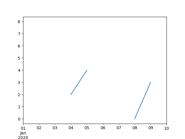
In [121]: ts Out[121]: 2020-01-01 8.0 2020-01-02 NaN 2020-01-03 NaN 2020-01-04 2.0 2020-01-05 4.0 2020-01-06 NaN 2020-01-07 NaN 2020-01-08 0.0 2020-01-09 3.0 2020-01-10 NaN Freq: D, dtype: float64
In [122]: ts.plot() Out[122]: <Axes: >
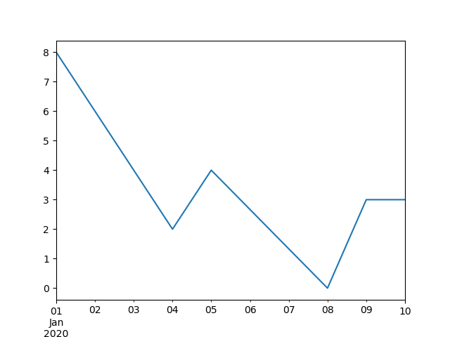
In [123]: ts.interpolate() Out[123]: 2020-01-01 8.000000 2020-01-02 6.000000 2020-01-03 4.000000 2020-01-04 2.000000 2020-01-05 4.000000 2020-01-06 2.666667 2020-01-07 1.333333 2020-01-08 0.000000 2020-01-09 3.000000 2020-01-10 3.000000 Freq: D, dtype: float64
In [124]: ts.interpolate().plot() Out[124]: <Axes: >
Interpolation relative to a Timestamp in the DatetimeIndexis available by setting method="time"
In [125]: ts2 = ts.iloc[[0, 1, 3, 7, 9]]
In [126]: ts2 Out[126]: 2020-01-01 8.0 2020-01-02 NaN 2020-01-04 2.0 2020-01-08 0.0 2020-01-10 NaN dtype: float64
In [127]: ts2.interpolate() Out[127]: 2020-01-01 8.0 2020-01-02 5.0 2020-01-04 2.0 2020-01-08 0.0 2020-01-10 0.0 dtype: float64
In [128]: ts2.interpolate(method="time") Out[128]: 2020-01-01 8.0 2020-01-02 6.0 2020-01-04 2.0 2020-01-08 0.0 2020-01-10 0.0 dtype: float64
For a floating-point index, use method='values':
In [129]: idx = [0.0, 1.0, 10.0]
In [130]: ser = pd.Series([0.0, np.nan, 10.0], idx)
In [131]: ser Out[131]: 0.0 0.0 1.0 NaN 10.0 10.0 dtype: float64
In [132]: ser.interpolate() Out[132]: 0.0 0.0 1.0 5.0 10.0 10.0 dtype: float64
In [133]: ser.interpolate(method="values") Out[133]: 0.0 0.0 1.0 1.0 10.0 10.0 dtype: float64
If you have scipy installed, you can pass the name of a 1-d interpolation routine to method. as specified in the scipy interpolation documentation and reference guide. The appropriate interpolation method will depend on the data type.
Tip
If you are dealing with a time series that is growing at an increasing rate, use method='barycentric'.
If you have values approximating a cumulative distribution function, use method='pchip'.
To fill missing values with goal of smooth plotting use method='akima'.
In [134]: df = pd.DataFrame( .....: { .....: "A": [1, 2.1, np.nan, 4.7, 5.6, 6.8], .....: "B": [0.25, np.nan, np.nan, 4, 12.2, 14.4], .....: } .....: ) .....:
In [135]: df Out[135]: A B 0 1.0 0.25 1 2.1 NaN 2 NaN NaN 3 4.7 4.00 4 5.6 12.20 5 6.8 14.40
In [136]: df.interpolate(method="barycentric") Out[136]: A B 0 1.00 0.250 1 2.10 -7.660 2 3.53 -4.515 3 4.70 4.000 4 5.60 12.200 5 6.80 14.400
In [137]: df.interpolate(method="pchip") Out[137]: A B 0 1.00000 0.250000 1 2.10000 0.672808 2 3.43454 1.928950 3 4.70000 4.000000 4 5.60000 12.200000 5 6.80000 14.400000
In [138]: df.interpolate(method="akima") Out[138]: A B 0 1.000000 0.250000 1 2.100000 -0.873316 2 3.406667 0.320034 3 4.700000 4.000000 4 5.600000 12.200000 5 6.800000 14.400000
When interpolating via a polynomial or spline approximation, you must also specify the degree or order of the approximation:
In [139]: df.interpolate(method="spline", order=2) Out[139]: A B 0 1.000000 0.250000 1 2.100000 -0.428598 2 3.404545 1.206900 3 4.700000 4.000000 4 5.600000 12.200000 5 6.800000 14.400000
In [140]: df.interpolate(method="polynomial", order=2) Out[140]: A B 0 1.000000 0.250000 1 2.100000 -2.703846 2 3.451351 -1.453846 3 4.700000 4.000000 4 5.600000 12.200000 5 6.800000 14.400000
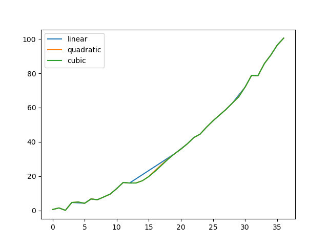
Comparing several methods.
In [141]: np.random.seed(2)
In [142]: ser = pd.Series(np.arange(1, 10.1, 0.25) ** 2 + np.random.randn(37))
In [143]: missing = np.array([4, 13, 14, 15, 16, 17, 18, 20, 29])
In [144]: ser.iloc[missing] = np.nan
In [145]: methods = ["linear", "quadratic", "cubic"]
In [146]: df = pd.DataFrame({m: ser.interpolate(method=m) for m in methods})
In [147]: df.plot() Out[147]: <Axes: >
Interpolating new observations from expanding data with Series.reindex().
In [148]: ser = pd.Series(np.sort(np.random.uniform(size=100)))
interpolate at new_index
In [149]: new_index = ser.index.union(pd.Index([49.25, 49.5, 49.75, 50.25, 50.5, 50.75]))
In [150]: interp_s = ser.reindex(new_index).interpolate(method="pchip")
In [151]: interp_s.loc[49:51] Out[151]: 49.00 0.471410 49.25 0.476841 49.50 0.481780 49.75 0.485998 50.00 0.489266 50.25 0.491814 50.50 0.493995 50.75 0.495763 51.00 0.497074 dtype: float64
Interpolation limits#
interpolate() accepts a limit keyword argument to limit the number of consecutive NaN values filled since the last valid observation
In [152]: ser = pd.Series([np.nan, np.nan, 5, np.nan, np.nan, np.nan, 13, np.nan, np.nan])
In [153]: ser Out[153]: 0 NaN 1 NaN 2 5.0 3 NaN 4 NaN 5 NaN 6 13.0 7 NaN 8 NaN dtype: float64
In [154]: ser.interpolate() Out[154]: 0 NaN 1 NaN 2 5.0 3 7.0 4 9.0 5 11.0 6 13.0 7 13.0 8 13.0 dtype: float64
In [155]: ser.interpolate(limit=1) Out[155]: 0 NaN 1 NaN 2 5.0 3 7.0 4 NaN 5 NaN 6 13.0 7 13.0 8 NaN dtype: float64
By default, NaN values are filled in a forward direction. Uselimit_direction parameter to fill backward or from both directions.
In [156]: ser.interpolate(limit=1, limit_direction="backward") Out[156]: 0 NaN 1 5.0 2 5.0 3 NaN 4 NaN 5 11.0 6 13.0 7 NaN 8 NaN dtype: float64
In [157]: ser.interpolate(limit=1, limit_direction="both") Out[157]: 0 NaN 1 5.0 2 5.0 3 7.0 4 NaN 5 11.0 6 13.0 7 13.0 8 NaN dtype: float64
In [158]: ser.interpolate(limit_direction="both") Out[158]: 0 5.0 1 5.0 2 5.0 3 7.0 4 9.0 5 11.0 6 13.0 7 13.0 8 13.0 dtype: float64
By default, NaN values are filled whether they are surrounded by existing valid values or outside existing valid values. The limit_areaparameter restricts filling to either inside or outside values.
fill one consecutive inside value in both directions
In [159]: ser.interpolate(limit_direction="both", limit_area="inside", limit=1) Out[159]: 0 NaN 1 NaN 2 5.0 3 7.0 4 NaN 5 11.0 6 13.0 7 NaN 8 NaN dtype: float64
fill all consecutive outside values backward
In [160]: ser.interpolate(limit_direction="backward", limit_area="outside") Out[160]: 0 5.0 1 5.0 2 5.0 3 NaN 4 NaN 5 NaN 6 13.0 7 NaN 8 NaN dtype: float64
fill all consecutive outside values in both directions
In [161]: ser.interpolate(limit_direction="both", limit_area="outside") Out[161]: 0 5.0 1 5.0 2 5.0 3 NaN 4 NaN 5 NaN 6 13.0 7 13.0 8 13.0 dtype: float64
Replacing values#
Series.replace() and DataFrame.replace() can be used similar toSeries.fillna() and DataFrame.fillna() to replace or insert missing values.
In [162]: df = pd.DataFrame(np.eye(3))
In [163]: df Out[163]: 0 1 2 0 1.0 0.0 0.0 1 0.0 1.0 0.0 2 0.0 0.0 1.0
In [164]: df_missing = df.replace(0, np.nan)
In [165]: df_missing Out[165]: 0 1 2 0 1.0 NaN NaN 1 NaN 1.0 NaN 2 NaN NaN 1.0
In [166]: df_filled = df_missing.replace(np.nan, 2)
In [167]: df_filled Out[167]: 0 1 2 0 1.0 2.0 2.0 1 2.0 1.0 2.0 2 2.0 2.0 1.0
Replacing more than one value is possible by passing a list.
In [168]: df_filled.replace([1, 44], [2, 28]) Out[168]: 0 1 2 0 2.0 2.0 2.0 1 2.0 2.0 2.0 2 2.0 2.0 2.0
Replacing using a mapping dict.
In [169]: df_filled.replace({1: 44, 2: 28}) Out[169]: 0 1 2 0 44.0 28.0 28.0 1 28.0 44.0 28.0 2 28.0 28.0 44.0
Regular expression replacement#
Note
Python strings prefixed with the r character such as r'hello world'are “raw” strings. They have different semantics regarding backslashes than strings without this prefix. Backslashes in raw strings will be interpreted as an escaped backslash, e.g., r'\' == '\\'.
Replace the ‘.’ with NaN
In [170]: d = {"a": list(range(4)), "b": list("ab.."), "c": ["a", "b", np.nan, "d"]}
In [171]: df = pd.DataFrame(d)
In [172]: df.replace(".", np.nan) Out[172]: a b c 0 0 a a 1 1 b b 2 2 NaN NaN 3 3 NaN d
Replace the ‘.’ with NaN with regular expression that removes surrounding whitespace
In [173]: df.replace(r"\s.\s", np.nan, regex=True) Out[173]: a b c 0 0 a a 1 1 b b 2 2 NaN NaN 3 3 NaN d
Replace with a list of regexes.
In [174]: df.replace([r".", r"(a)"], ["dot", r"\1stuff"], regex=True) Out[174]: a b c 0 0 astuff astuff 1 1 b b 2 2 dot NaN 3 3 dot d
Replace with a regex in a mapping dict.
In [175]: df.replace({"b": r"\s.\s"}, {"b": np.nan}, regex=True) Out[175]: a b c 0 0 a a 1 1 b b 2 2 NaN NaN 3 3 NaN d
Pass nested dictionaries of regular expressions that use the regex keyword.
In [176]: df.replace({"b": {"b": r""}}, regex=True) Out[176]: a b c 0 0 a a 1 1 b 2 2 . NaN 3 3 . d
In [177]: df.replace(regex={"b": {r"\s.\s": np.nan}}) Out[177]: a b c 0 0 a a 1 1 b b 2 2 NaN NaN 3 3 NaN d
In [178]: df.replace({"b": r"\s*(.)\s*"}, {"b": r"\1ty"}, regex=True) Out[178]: a b c 0 0 a a 1 1 b b 2 2 .ty NaN 3 3 .ty d
Pass a list of regular expressions that will replace matches with a scalar.
In [179]: df.replace([r"\s.\s", r"a|b"], "placeholder", regex=True) Out[179]: a b c 0 0 placeholder placeholder 1 1 placeholder placeholder 2 2 placeholder NaN 3 3 placeholder d
All of the regular expression examples can also be passed with theto_replace argument as the regex argument. In this case the valueargument must be passed explicitly by name or regex must be a nested dictionary.
In [180]: df.replace(regex=[r"\s.\s", r"a|b"], value="placeholder") Out[180]: a b c 0 0 placeholder placeholder 1 1 placeholder placeholder 2 2 placeholder NaN 3 3 placeholder d
Note
A regular expression object from re.compile is a valid input as well.