dsp.SOSFilter - Implement cascade of second order section filters - MATLAB (original) (raw)
Implement cascade of second order section filters
Description
The dsp.SOSFilter System object™ implements an IIR filter structure using second-order sections (SOS).
To implement an IIR filter structure using SOS:
- Create the
dsp.SOSFilterobject and set its properties. - Call the object with arguments, as if it were a function.
To learn more about how System objects work, see What Are System Objects?
This object supports C/C++ code generation and SIMD code generation under certain conditions. This object also supports code generation for ARM® Cortex®-M and ARM Cortex-A processors. For more information, see Code Generation.
Creation
Syntax
Description
`sos` = dsp.SOSFilter returns a biquadratic IIR filter System object, sos, which independently filters each channel (column) of the input over time using a specified biquadratic structure.
`sos` = dsp.SOSFilter(`num`,`den`) returns a biquadratic filter object with the Numerator property set to num and the Denominator property set toden.
`sos` = dsp.SOSFilter(`Name,Value`) returns a biquadratic filter object with each property set to the specified value. Enclose each property name in single quotes.
Example: sos = dsp.SOSFilter('CoefficientSource','Input port')
Properties
Unless otherwise indicated, properties are nontunable, which means you cannot change their values after calling the object. Objects lock when you call them, and therelease function unlocks them.
If a property is tunable, you can change its value at any time.
For more information on changing property values, seeSystem Design in MATLAB Using System Objects.
Filter structure, specified as one of 'Direct form I','Direct form I transposed', 'Direct form II', or'Direct form II transposed'.
Source of the filter coefficients, specified as one of the following:
'Property'–– The filter coefficients are specified through theNumerator,Denominator, andScaleValuesproperties.'Input port'–– The numerator coefficients, denominator coefficients, and the scale values are specified as inputs to the object while running the algorithm. For more details, see Usage.
Numerator coefficients of the filter, specified as an _P_-by-3 matrix, where P is the number of biquadratic sections. Each row corresponds to the numerator coefficients of the corresponding section of the filter.
The size of this property cannot be modified once you have run the System object algorithm. However, the coefficient values can change as the property is tunable.
Tunable: Yes
Dependencies
To enable this property, set the CoefficientSource property to 'Property'.
Data Types: single | double | int8 | int16 | int32 | int64 | uint8 | uint16 | uint32 | uint64
Complex Number Support: Yes
Denominator coefficients of the filter, specified as an _P_-by-3 matrix, where P is the number of biquadratic sections. Each row corresponds to the denominator coefficients of the corresponding section of the filter.
The leading denominator coefficient is always assumed to be 1. If any other value is specified in the first column, the object ignores this value and treats it as 1.
The size of this property cannot be modified once you step through the algorithm. However, the denominator values can be modified as the property is tunable.
Tunable: Yes
Dependencies
To enable this property, set CoefficientSource property to'Property'.
Data Types: single | double | int8 | int16 | int32 | int64 | uint8 | uint16 | uint32 | uint64
Complex Number Support: Yes
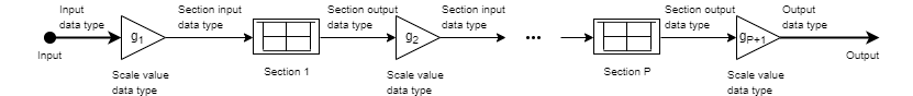
Specify if the filter has scale values for each section. When set totrue, using the ScaleValues property, you can specify the scale values to be applied before and after each section of the biquadratic filter.
Scale values to apply before and after each section of a biquadratic filter, specified as a vector. The length of the ScaleValues vector must be P + 1, where P is the number of biquadratic sections. If you set this property to a scalar value, the scalar value is used as the gain value only before the first filter section. The remaining gain values are set to 1. If you set this property to a vector of_P_ + 1 values, each value is used for a separate section of the filter.
Tunable: Yes
Dependencies
This property applies only when you set the CoefficientSource property to 'Property' and HasScaleValues property to true.
Data Types: single | double | int8 | int16 | int32 | int64 | uint8 | uint16 | uint32 | uint64
Fixed-Point Properties
Rounding method for fixed-point operations, specified as one of the following:
'Floor''Ceiling''Convergent''Nearest''Round''Simplest''Zero'
For more details, see Rounding Modes.
Overflow action for fixed-point operations, specified as one of the following:
'Wrap'–– The object wraps the result of its fixed-point operations.'Saturate'–– The object saturates the result of its fixed-point operations.
For more details on overflow actions, see Overflow Handling for fixed-point operations.
Section input word- and fraction-length designations, specified as either'Same as input' or a numerictype (Fixed-Point Designer) object.
When specified as a numerictype object, the data type must be signed fixed point with a power-of-two slope and zero bias.
Dependencies
This property applies only when you set the HasScaleValues property to true.
Section output word- and fraction-length designations, specified as either'Same as section input' or a numerictype (Fixed-Point Designer) object.
When specified as a numerictype object, the data type must be signed fixed point with a power-of-two slope and zero bias.
Dependencies
This property applies only when you set the HasScaleValues property to true.
Numerator coefficients word- and fraction-length designations, specified as either'Same word length as input' or as anumerictype object.
When specified as a numerictype object, the data type must be signed fixed point with a power-of-two slope and zero bias. If not specified, the fraction length is determined based on the numerator coefficient values to give the best possible precision.
Dependencies
This property applies only when you set theCoefficientSource property to'Property'.
Denominator coefficients word- and fraction-length designations, specified as either 'Same word length as input' or as anumerictype object.
When specified as a numerictype object, the data type must be signed fixed point with a power-of-two slope and zero bias. If not specified, the fraction length is determined based on the denominator coefficient values to give the best possible precision.
Dependencies
This property applies only when you set theCoefficientSource property to'Property'.
Scale values word- and fraction-length designations, specified as either'Same word length as input' or as anumerictype object.
When specified as a numerictype object, the data type must be signed fixed point with a power-of-two slope and zero bias. If not specified, the fraction length is determined based on the scale values to give the best possible precision.
Dependencies
This property applies only when you set theCoefficientSource property to 'Property' and HasScaleValues property to true.
Multiplicand word- and fraction-length designations, specified as either'Same as output' or as a numerictype object.
When specified as a numerictype object, the data type must be signed fixed point with a power-of-two slope and zero bias.
Dependencies
This property applies only when you set the Structure property to 'Direct form I transposed'.
State word- and fraction-length designations, specified as either 'Full precision' or as a numerictype object.
When specified as a numerictype object, the data type must be signed fixed point with a power-of-two slope and zero bias.
Dependencies
This property applies only when you set the Structure property to 'Direct form II'.
Denominator accumulator word- and fraction-length designations, specified as anumerictype object.
Output word- and fraction-length designations, specified as either 'Full precision' or as a numerictype object. When specified as a numerictype object, the data type must be signed fixed point with a power-of-two slope and zero bias.
When the input is floating-point, the output data type matches the input data type since floating-point inheritance takes precedence over the fixed-point settings.
Usage
Syntax
Description
[y](#mw%5Fe9d84a56-e345-4139-a6b9-c569970b4446) = sos([x](#mw%5F6bcbfc68-7848-48b0-ace5-43c7aa8a74fb)) filters the input signal x and outputs the filtered valuesy. The sos filter object filters each channel (column) of the input signal independently over successive calls to the algorithm.
This syntax is valid only when the CoefficientSource property is set to 'Property'.
[y](#mw%5Fe9d84a56-e345-4139-a6b9-c569970b4446) = sos([x](#mw%5F6bcbfc68-7848-48b0-ace5-43c7aa8a74fb),[num](#mw%5Ffe272671-c8f1-45f3-a3ce-b8a546e843a2),[den](#mw%5F0c61761a-f252-400e-9951-5320fd325eed)) filters the input using num as the numerator coefficients andden as the denominator coefficients of the sos filter.
This syntax is valid only when the CoefficientSource property is set to 'Input port' and HasScaleValues property is set to false.
[y](#mw%5Fe9d84a56-e345-4139-a6b9-c569970b4446) = sos([x](#mw%5F6bcbfc68-7848-48b0-ace5-43c7aa8a74fb),[num](#mw%5Ffe272671-c8f1-45f3-a3ce-b8a546e843a2),[den](#mw%5F0c61761a-f252-400e-9951-5320fd325eed),[g](#mw%5F4984ea09-b4df-4876-9e1f-12840771ee5d)) specifies the scale values g of the sos filter.
This syntax is valid only when the CoefficientSource property is set to 'Input port' and HasScaleValues property is set to true.
Input Arguments
Data input, specified as a vector or a matrix.
This object also accepts variable-size inputs. Once you have run the System object algorithm, you can change the size of each input channel, but you cannot change the number of channels.
If the input is fixed-point, it must be signed fixed point with a power-of-two slope and zero bias. When the fraction length is not specified, the object determines the fraction length based on the input data to give the best possible precision.
The data type of all inputs must be the same.
Data Types: single | double | int8 | int16 | int32 | int64 | fi
Complex Number Support: Yes
Numerator coefficients, specified as an P_-by-3 matrix, where_P is the number of biquadratic sections. Each row corresponds to the numerator coefficients of the corresponding section of the filter.
Once you step through the algorithm, the size of this input cannot be modified. However, the numerator coefficient values can be modified as the input is tunable.
If num is fixed-point, it must be signed fixed point with a power-of-two slope and zero bias. When the fraction length is not specified, the object determines the fraction length based on the numerator coefficient values to give the best possible precision.
The data type of all inputs must be the same.
The size and complexity of the num andden inputs must be the same.
Tunable: Yes
Dependencies
This input applies only when you set the CoefficientSource property to 'Input port'.
Data Types: single | double | int8 | int16 | int32 | int64 | fi
Complex Number Support: Yes
Denominator coefficients of the filter, specified as an _P_-by-3 matrix, where P is the number of biquadratic sections. Each row corresponds to the denominator coefficients of the corresponding section of the filter.
The leading denominator coefficient is always assumed to be 1. If any other value is specified in the first column, the object ignores this value and treats it as 1.
The size of this input cannot be modified once you step through the algorithm. However, the denominator values can be modified as the input is tunable.
If den is fixed-point, it must be signed fixed point with a power-of-two slope and zero bias. When the fraction length is not specified, the object determines the fraction length based on the denominator coefficient values to give the best possible precision.
The data type of all inputs must be the same.
The size and complexity of the num andden inputs must be the same.
Tunable: Yes
Dependencies
This input applies only when you set the CoefficientSource property to 'Input port'.
Data Types: single | double | int8 | int16 | int32 | int64 | fi
Complex Number Support: Yes
Scale values of the biquadratic filter, specified as a 1-by-(P+1) vector, where P is the number of biquadratic filter sections.
If g is fixed-point, it must be signed fixed point with a power-of-two slope and zero bias. When the fraction length is not specified, the object determines the fraction length based on the scale values to give the best possible precision.
The data type of all inputs must be the same.
Tunable: Yes
Dependencies
This input applies only when you set the CoefficientSource property to 'Input port' and HasScaleValues property to true.
Data Types: single | double | int8 | int16 | int32 | int64 | fi
Output Arguments
Filtered output, returned as a vector or a matrix. The size and complexity of the output signal matches that of the input signal.
When the input is fixed-point, the data type of the output is determined based on the value of the OutputDataType property. If you setOutputDataType to 'Full precision', the output data type is computed based on the signal flow diagrams shown in the Fixed-Point Conversion section. If you set OutputDataType to a custom numeric type, the output data type is cast to the specified numeric type.
When the input is floating-point, the output data type matches the input data type since floating-point inheritance takes precedence over the fixed-point settings.
Data Types: single | double | int8 | int16 | int32 | int64 | fi
Complex Number Support: Yes
Object Functions
To use an object function, specify the System object as the first input argument. For example, to release system resources of a System object named obj, use this syntax:
| freqz | Frequency response of discrete-time filter System object |
|---|---|
| filterAnalyzer | Analyze filters with Filter Analyzer app |
| impz | Impulse response of discrete-time filter System object |
| info | Information about filter System object |
| coeffs | Returns the filter System object coefficients in a structure |
| cost | Estimate cost of implementing filter System object |
| scale | Scale second-order sections |
| scaleopts | Create an options object for second-order section scaling |
| scalecheck | Check scaling of biquadratic filter |
| cumsec | Cumulative second-order section of the biquadratic filter |
| tf | Convert discrete-time filter System object to transfer function |
| reorder | Reorder second-order sections of biquadratic filter System object |
| outputDelay | Determine output delay of single-rate or multirate filter |
| step | Run System object algorithm |
|---|---|
| release | Release resources and allow changes to System object property values and input characteristics |
| reset | Reset internal states of System object |
Examples
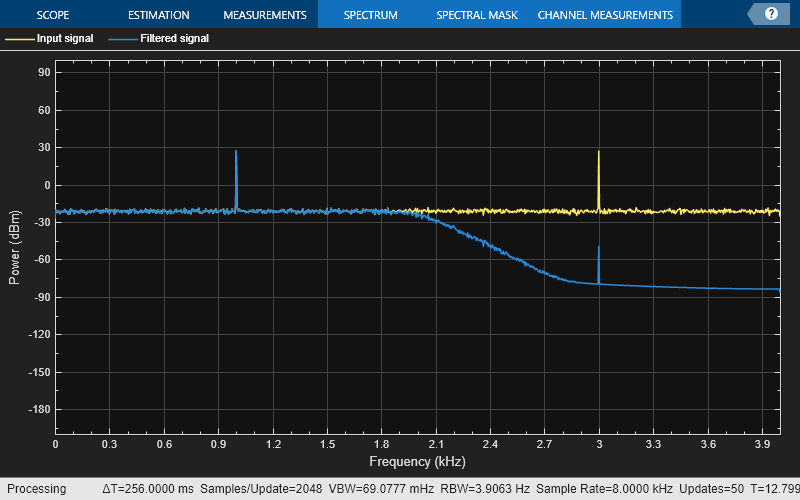
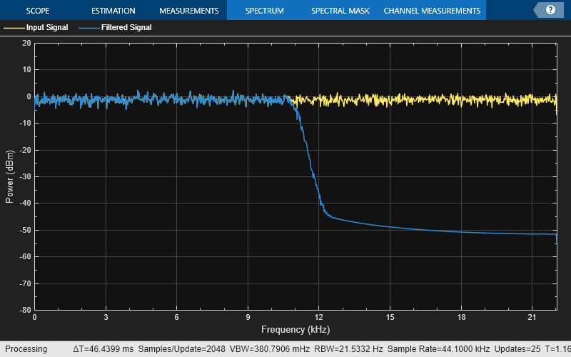
Lowpass filter a noisy sinusoidal signal using the dsp.SOSFilter System object. Visualize the original and filtered signals using a spectrum analyzer.
Input Signal
The input signal is a sinusoidal signal with two tones, one at 1 kHz and the other at 3 kHz. The sampling frequency is 8 kHz.
f1 = 1000; f2 = 3000; Fs = 8000; sine = dsp.SineWave(Frequency=[f1,f2],... SampleRate=Fs,... SamplesPerFrame=1024);
Create Biquad SOS Filter
Design a 10th-order lowpass Butterworth IIR filter with a cutoff frequency of 2 kHz. The numerator and denominator coefficients are extracted from the designed SOS matrix.
Fcutoff = 2000; [z,p,k] = butter(10,Fcutoff/(Fs/2)); [s, g] = zp2sos(z,p,k); [num,den] = sos2ctf(s);
sosFilter = dsp.SOSFilter(num,den,... ScaleValues=g)
sosFilter = dsp.SOSFilter with properties:
        Structure: 'Direct form II transposed'
CoefficientSource: 'Property'
        Numerator: [5×3 double]
      Denominator: [5×3 double]
   HasScaleValues: true
      ScaleValues: [0.0029 1 1 1 1 1]
Show all properties
Visualize the frequency response of the designed SOS filter.
Streaming
Add zero-mean white Gaussian noise with a standard deviation of 0.1 to the sum of sine waves. Filter the noisy sinusoidal signal with the designed SOS filter.
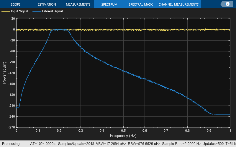
While running the simulation, the spectrum analyzer shows that the high-frequency tone above 2 kHz in the source signal is attenuated. The resulting signal maintains the peak at 1 kHz because it falls in the passband of the lowpass filter.
SA = spectrumAnalyzer(... PlotAsTwoSidedSpectrum=false, ... SampleRate=Fs, ... ShowLegend=true,... YLimits=[-200 100],... ChannelNames={'Input signal','Filtered signal'});
% Stream processing loopfor k = 1:100 input = sum(sine(),2) + 0.1.*randn(sine.SamplesPerFrame,1); filteredOutput = sosFilter(input); SA(input,filteredOutput); end
Design a lowpass biquadratic SOS filter with time-varying coefficients. Visualize the magnitude response of the filter using a dynamic filter visualizer.
dfv = dsp.DynamicFilterVisualizer('YLimits',[-120 10])
dfv = dsp.DynamicFilterVisualizer handle with properties:
           FFTLength: 2048
 NormalizedFrequency: 0
          SampleRate: 44100
      FrequencyRange: [0 22050]
              XScale: 'Linear'
    MagnitudeDisplay: 'Magnitude (dB)'
PlotAsMagnitudePhase: 0
         AxesScaling: 'Manual'
Show all properties
Create a dsp.SOSFilter object.
sosfilt = dsp.SOSFilter with properties:
        Structure: 'Direct form II transposed'
CoefficientSource: 'Property'
        Numerator: [0.0975 0.1950 0.0975]
      Denominator: [1 -0.9428 0.3333]
   HasScaleValues: false
Show all properties
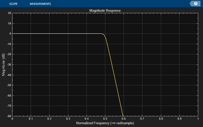
Use the maxflat function to design a lowpass maximally flat filter. Set the numerator and denominator order of the filter to 2 since the SOS filter is biquadratic. Vary the cutoff frequency in 0.001 increments and design the filter for each increment. Pass the computed coefficients to the SOS filter. Visualize the time-varying magnitude response of the SOS filter using the dsp.DynamicFilterVisualizer object.
for Wn = 0.1:0.001:0.6 [b,a] = maxflat(2,2,Wn); sosfilt.Numerator = b; sosfilt.Denominator = a; dfv(sosfilt) end
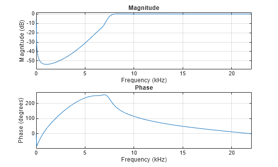
Design a peak filter of order 14 and a center frequency at 0.2 rad/s using the designNotchPeakIIR function. Output scale values by setting the HasScaleValues property to true.
[b,a,sv] = designNotchPeakIIR(FilterOrder=14, CenterFrequency=0.2,... HasScaleValues=true)
b = 7×3
1.0000    2.0000    1.0000
1.0000   -2.0000    1.0000
1.0000    2.0000    1.0000
1.0000   -2.0000    1.0000
1.0000    2.0000    1.0000
1.0000   -2.0000    1.0000
1.0000         0   -1.0000
a = 7×3
1.0000   -1.4026    0.9374
1.0000   -1.7004    0.9549
1.0000   -1.3637    0.8373
1.0000   -1.6111    0.8736
1.0000   -1.3788    0.7823
1.0000   -1.5195    0.8103
1.0000   -1.4366    0.7757
sv = 8×1
0.1220
0.1220
0.1166
0.1166
0.1133
0.1133
0.1122
1.0000
Assign the filter design coefficients to a dsp.SOSFilter object.
peakFilter = dsp.SOSFilter(b,a,ScaleValues=sv)
peakFilter = dsp.SOSFilter with properties:
        Structure: 'Direct form II transposed'
CoefficientSource: 'Property'
        Numerator: [7×3 double]
      Denominator: [7×3 double]
   HasScaleValues: true
      ScaleValues: [8×1 double]
Show all properties
Create a dsp.DynamicFilterVisualizer object to display the magnitude response of the filter.
dfv = dsp.DynamicFilterVisualizer(NormalizedFrequency=true); dfv(peakFilter)
Create a spectrumAnalyzer object to visualize the input and output spectra.
scope = spectrumAnalyzer(SampleRate=2,PlotAsTwoSidedSpectrum=false,... ChannelNames=["Input Signal","Filtered Signal"]);
Stream in random data and filter the signal using the peak filter you have designed.
for i = 1:1000 x = randn(1024, 1); y = peakFilter(x); scope(x,y); end
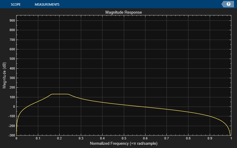
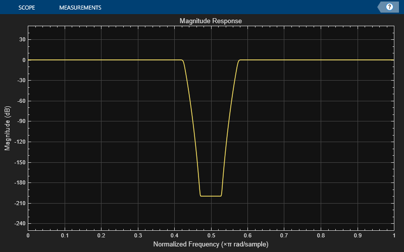
Design a notch filter object of order 48 and a bandwidth of 0.15 using the designNotchPeakIIR function.
notchFilter = designNotchPeakIIR(FilterOrder=48,Bandwidth=0.15,... Response='notch',SystemObject=true)
notchFilter = dsp.SOSFilter with properties:
        Structure: 'Direct form II transposed'
CoefficientSource: 'Property'
        Numerator: [24×3 double]
      Denominator: [24×3 double]
   HasScaleValues: false
Show all properties
Create a dsp.DynamicFilterVisualizer object to display the magnitude response of the filter.
dfv = dsp.DynamicFilterVisualizer(NormalizedFrequency=true,YLimits=[-250 50]); dfv(notchFilter)
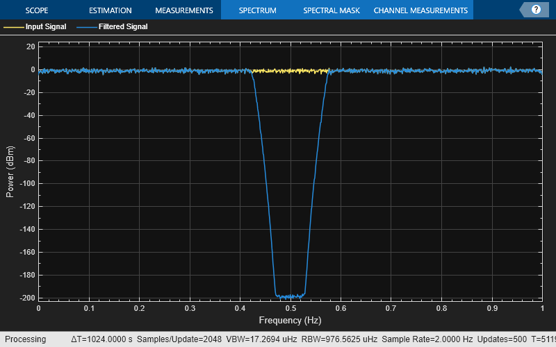
Create a spectrumAnalyzer object to visualize the input and output spectra.
scope = spectrumAnalyzer(SampleRate=2,PlotAsTwoSidedSpectrum=false,... ChannelNames=["Input Signal","Filtered Signal"]);
Stream in random data and filter the signal using the notch filter.
for i = 1:1000 x = randn(1024, 1); y = notchFilter(x); scope(x,y); end
Create a dsp.SOSFilter object, and set the CoefficientSource property to 'Input port' so that you can vary the coefficients of the SOS filter coefficients through the input port during simulation.
sosFilt = dsp.SOSFilter(CoefficientSource="Input port")
sosFilt = dsp.SOSFilter with properties:
        Structure: 'Direct form II transposed'
CoefficientSource: 'Input port'
   HasScaleValues: false
Show all properties
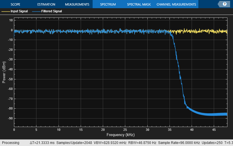
Create a spectrumAnalyzer object to visualize the spectra of the input and output signals.
spectrumScope = spectrumAnalyzer(SampleRate=96000,PlotAsTwoSidedSpectrum=false,... ChannelNames=["Input Signal","Filtered Signal"]);
Create a dsp.DynamicFilterVisualizer object to visualize the magnitude response of the varying filter.
filterViz = dsp.DynamicFilterVisualizer(NormalizedFrequency=true);
Stream in random data and filter the signal using the dsp.SOSFilter object. Use the designLowpassIIR function to design the filter coefficients. By default, this function returns a _P_-by-3 matrix of numerator coefficients and a _P_-by-3 matrix of denominator coefficients. Assign these coefficients to the dsp.SOSFilter object.
Vary the 3-dB cutoff frequency of the filter during simulation. The designLowpassIIR function redesigns the coefficients based on the updated filter specifications. Pass these updated coefficients to the SOS filter. Visualize the spectra of the input and filtered signals using the spectrum analyzer.
F3dB = 0.5; for idx = 1:500 [b,a] = designLowpassIIR(FilterOrder=30,HalfPowerFrequency=F3dB,DesignMethod="butter"); x = randn(1024,1); y = sosFilt(x,b,a); spectrumScope(x,y); filterViz(b,a); F3dB = F3dB + 0.0005; end
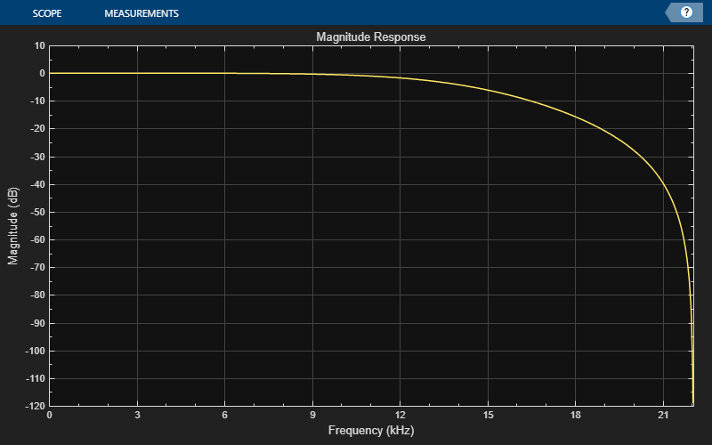
Design and implement a lowpass IIR filter object using the designLowpassIIR function. The function returns a dsp.SOSFilter object when you set the SystemObject argument to true. To design the filter in single-precision, use the Datatype or like argument. Alternatively, you can specify any of the numerical arguments in single-precision.
sosFilt = designLowpassIIR(FilterOrder=30,HalfPowerFrequency=0.5,DesignMethod="butter",... Datatype="single",SystemObject=true)
sosFilt = dsp.SOSFilter with properties:
        Structure: 'Direct form II transposed'
CoefficientSource: 'Property'
        Numerator: [15×3 single]
      Denominator: [15×3 single]
   HasScaleValues: false
Show all properties
Create a dsp.DynamicFilterVisualizer object to visualize the magnitude response of the filter.
filterViz = dsp.DynamicFilterVisualizer(NormalizedFrequency=true,YLimits=[-80 20]); filterViz(sosFilt)
Create a spectrumAnalyzer object to visualize the spectra of the input and output signals.
spectrumScope = spectrumAnalyzer(SampleRate=44100,PlotAsTwoSidedSpectrum=false,... ChannelNames=["Input Signal","Filtered Signal"]);
Stream in random data and filter the signal using the dsp.SOSFilter object. Visualize the spectra of the input and filtered signals using the spectrum analyzer.
for idx = 1:50 x = randn(1024,1); y = sosFilt(x); spectrumScope(x,y); end
Since R2023b
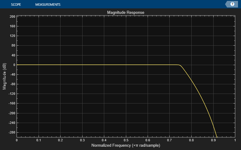
Design a highpass IIR filter using the designfilt function.
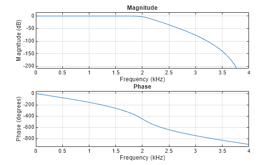
The filter is a 20th order highpass IIR filter with a sample rate of 44.1 kHz. The stopband frequency of the filter is 3 kHz and the passband frequency is 8 kHz. Use the IIR least p-norm design method and set the _L_-infinity norm to 120. Set the SystemObject argument to true.
With these specifications, the designfilt function generates a dsp.SOSFilter System object™.
hpIIRFilter = designfilt('highpassiir', ... FilterOrder=20,StopbandFrequency=3000, ... PassbandFrequency=8000,SampleRate=44100, ... Norm=120,SystemObject=true)
hpIIRFilter = dsp.SOSFilter with properties:
        Structure: 'Direct form II'
CoefficientSource: 'Property'
        Numerator: [10×3 double]
      Denominator: [10×3 double]
   HasScaleValues: true
      ScaleValues: [0.5812 1 1 1 1 1 1 1 1 1 14.8291]
Show all properties
Visualize the frequency response of this filter.
freqz(hpIIRFilter,[],44100)
More About
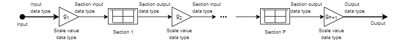
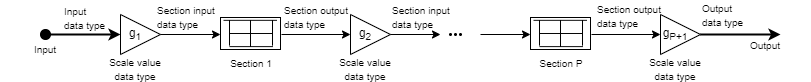
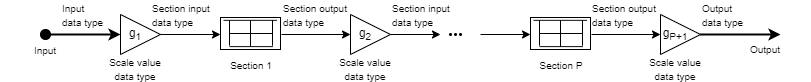
These diagrams show the filter structures supported by the second-order section filter.
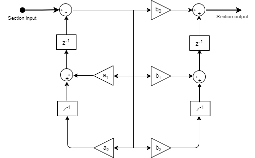
Direct Form I
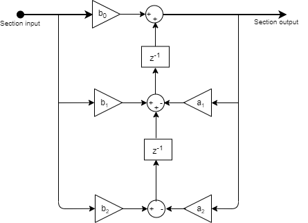
This is the structure of each section in the filter when you set the filter structure toDirect form I.

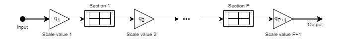
This is the structure of the filter with P sections when you specify scale values [_g_1,_g_2, …,_g_P+1].
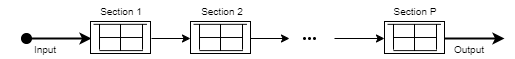
This is the structure of the filter when you do not specify scale values.
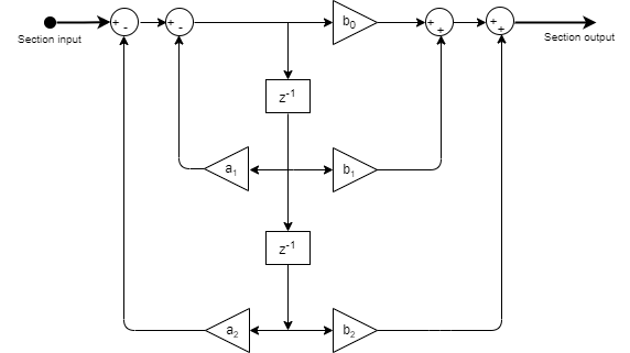
Direct Form I Transposed
This is the structure of each section in the filter when you set the filter structure toDirect form I transposed.
This is the structure of the filter with P sections when you specify scale values [_g_1,_g_2, …,_g_P+1].
This is the structure of the filter when you do not specify scale values.
Direct Form II
This is the structure of each section in the filter when you set the filter structure toDirect form II.
This is the structure of the filter with P sections when you specify scale values [_g_1,_g_2, …,_g_P+1].
This is the structure of the filter when you do not specify scale values.
Direct Form II Transposed
This is the structure of each section in the filter when you set the filter structure toDirect form II transposed.
This is the structure of the filter with P sections when you specify scale values [_g_1,_g_2, …,_g_P+1].
This is the structure of the filter when you do not specify scale values.
These diagrams show the data types used in the SOS filter when the input is fixed-point. For each structure the filter supports, the data types shown in the diagrams can be set through the respective fixed-point settings.
Direct Form I
Here is the structure of each section when you set the filter structure toDirect form I. This diagram shows the data types when you input fixed-point signals. The gain operations_b0_,b1,b2,a1, and_a2_ operate in full precision.
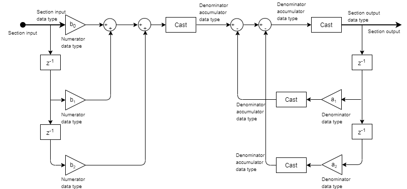
These diagrams show the fixed-point data types between filter sections.
When the data is not optimized:
When you specify scale values to 1:

Direct Form I Transposed
Here is the structure of each section when you set the filter structure toDirect form I transposed. This diagram shows the data types when you input fixed-point signals. The dashed casts are omitted when you setHasScaleValues to false. The gain operations_b0_,b1,b2,a1, and_a2_ operate in full precision.
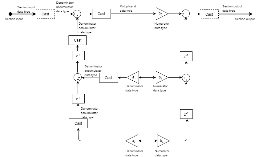
These diagrams show the fixed-point data types between filter sections.
When the data is not optimized:
When you specify scale values to 1:

Direct Form II
Here is the structure of each section when you set the filter structure toDirect form II. This diagram shows the data types when you input fixed-point signals. The dashed casts are omitted when you setHasScaleValues to false. The gain operations_b0_,b1,b2,a1, and_a2_ operate in full precision.
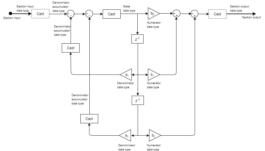
These diagrams show the fixed-point data types between filter sections.
When the data is not optimized:
When you set scale values to 1:

Direct Form II Transposed
Here is the structure of each section when you set the filter structure toDirect form II transposed. This diagram shows the data types when you input fixed-point signals. The gain operations_b0_,b1,b2,a1, and_a2_ operate in full precision. When you setHasScaleValues to false, the data type at the section output is automatically determined by the object algorithm and is not controlled by the value of the SectionOutputDataType property.

These diagrams show the fixed-point data types between filter sections.
When the data is not optimized:
When you specify scale values to 1:

Extended Capabilities
Usage notes and limitations:
See System Objects in MATLAB Code Generation (MATLAB Coder).
The dsp.SOSFilter System object supports optimized C code generation on ARM Cortex-M processors and SIMD code generation under these conditions:
- Input is a single-channel real-valued signal.
- Data type of the input is
single. - When you set
Structureto'Direct form I'or'Direct form II transposed'. - When you set
HasScaleValuestofalse.
In the case of code generation for ARM Cortex-M processors, setHasScaleValuestofalseafter settingCoefficientSourceto'Input port'.
The SIMD technology significantly improves the performance of the generated code. For more information, see SIMD Code Generation. To generate SIMD code from this object, see Use Intel AVX2 Code Replacement Library to Generate SIMD Code from MATLAB Algorithms.
Version History
Introduced in R2020a
The designfilt function generates adsp.SOSFilter object when you specify 'lowpassiir' and 'highpassiir' filter responses and set the'SystemObject' flag to 'true'.
hpIIRFilter = designfilt('highpassiir', ... 'FilterOrder',20,'StopbandFrequency',3000, ... 'PassbandFrequency',8000,'SampleRate',44100, ... 'Norm',120,'SystemObject',true)
hpIIRFilter = dsp.SOSFilter with properties:
        Structure: 'Direct form II'
CoefficientSource: 'Property'
        Numerator: [10×3 double]
      Denominator: [10×3 double]
   HasScaleValues: true
      ScaleValues: [0.4745 1 1 1 1 1 1 1 1 1 1.6434]
The Design Filter Live Editor task generates a dsp.SOSFilter object for lowpass IIR and highpass IIR filter responses when you select the Use a System object to implement filter check box in the task UI and run thedesignfilt code the task generates.
In R2022b, you can generate optimized C code for the dsp.SOSFilter object on ARM Cortex-M processors under certain conditions. For more details, see Code Generation.
See Also
Functions
- freqz | filterAnalyzer | impz | info | coeffs | cost | scale | scaleopts | scalecheck | cumsec | tf | scaleFilterSections | outputDelay | designLowpassIIR | designHighpassIIR | designBandpassIIR | designBandstopIIR | designNotchPeakIIR