accelerate - (Not recommended) Option to accelerate computation of gradient for approximator
object based on neural network - MATLAB ([original](https://www.mathworks.com/help/reinforcement-learning/ref/rl.function.rlcontinuousdeterministicactor.accelerate.html)) ([raw](?raw))(Not recommended) Option to accelerate computation of gradient for approximator object based on neural network
Since R2022a
Syntax
Description
[newAppx](#mw%5Fd91da2d6-accf-424e-8151-007e8082f56b) = accelerate([oldAppx](#mw%5F812a2ed6-d7b8-4bb0-b5bf-ece06052518e),[useAcceleration](#mw%5Faefd9e92-f777-4eda-8d17-6fec0ea7610b)) returns the new neural-network-based function approximator objectnewAppx, which has the same configuration as the original object,oldAppx, and the option to accelerate the gradient computation set to the logical value useAcceleration.
Examples
Accelerate Gradient Computation for a Q-Value Function
Create observation and action specification objects (or alternatively use getObservationInfo andgetActionInfo to extract the specification objects from an environment). For this example, define an observation space with two channels. The first channel carries an observation from a continuous four-dimensional space. The second carries a discrete scalar observation that can be either zero or one. Finally, the action space is a three-dimensional vector in a continuous action space.
obsInfo = [rlNumericSpec([4 1]) rlFiniteSetSpec([0 1])];
actInfo = rlNumericSpec([3 1]);
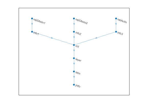
To approximate the Q-value function within the critic, create a recurrent deep neural network. The output layer must be a scalar expressing the value of executing the action given the observation.
Define each network path as an array of layer objects. Get the dimensions of the observation and action spaces from the environment specification objects, and specify a name for the input layers, so you can later explicitly associate them with the appropriate environment channel. Since the network is recurrent, usesequenceInputLayer as the input layer and include anlstmLayer as one of the other network layers.
% Define paths inPath1 = [ sequenceInputLayer( ... prod(obsInfo(1).Dimension), ... Name="netObsIn1") fullyConnectedLayer(5,Name="infc1") ];
inPath2 = [ sequenceInputLayer( ... prod(obsInfo(2).Dimension), ... Name="netObsIn2") fullyConnectedLayer(5,Name="infc2") ];
inPath3 = [ sequenceInputLayer( ... prod(actInfo(1).Dimension), ... Name="netActIn") fullyConnectedLayer(5,Name="infc3") ];
% Concatenate 3 previous layer outputs along dim 1 jointPath = [ concatenationLayer(1,3,Name="cct") tanhLayer lstmLayer(8,"OutputMode","sequence") fullyConnectedLayer(1,Name="jntfc") ];
Assemble dlnetwork object.
net = dlnetwork; net = addLayers(net,inPath1); net = addLayers(net,inPath2); net = addLayers(net,inPath3); net = addLayers(net,jointPath);
Connect layers.
net = connectLayers(net,"infc1","cct/in1"); net = connectLayers(net,"infc2","cct/in2"); net = connectLayers(net,"infc3","cct/in3");
Plot network.
Initialize network and display the number of weights.
net = initialize(net); summary(net)
Initialized: true
Number of learnables: 832
Inputs: 1 'netObsIn1' Sequence input with 4 dimensions 2 'netObsIn2' Sequence input with 1 dimensions 3 'netActIn' Sequence input with 3 dimensions
Create the critic with rlQValueFunction, using the network, and the observation and action specification objects.
critic = rlQValueFunction(net, ... obsInfo, ... actInfo, ... ObservationInputNames=["netObsIn1","netObsIn2"], ... ActionInputNames="netActIn");
To return the value of the actions as a function of the current observation, usegetValue or evaluate.
val = evaluate(critic, ... { rand(obsInfo(1).Dimension), ... rand(obsInfo(2).Dimension), ... rand(actInfo(1).Dimension) })
val = 1×1 cell array {[0.0089]}
When you use evaluate, the result is a single-element cell array containing the value of the action in the input, given the observation.
Calculate the gradients of the sum of the three outputs with respect to the inputs, given a random observation.
gro = gradient(critic,"output-input", ... { rand(obsInfo(1).Dimension) , ... rand(obsInfo(2).Dimension) , ... rand(actInfo(1).Dimension) } )
gro=3×1 cell array {4×1 single} {[ -0.0945]} {3×1 single}
The result is a cell array with as many elements as the number of input channels. Each element contains the derivatives of the sum of the outputs with respect to each component of the input channel. Display the gradient with respect to the element of the second channel.
Obtain the gradient with respect of five independent sequences, each one made of nine sequential observations.
gro_batch = gradient(critic,"output-input", ... { rand([obsInfo(1).Dimension 5 9]) , ... rand([obsInfo(2).Dimension 5 9]) , ... rand([actInfo(1).Dimension 5 9]) } )
gro_batch=3×1 cell array {4×1×5×9 single} {1×1×5×9 single} {3×1×5×9 single}
Display the derivative of the sum of the outputs with respect to the third observation element of the first input channel, after the seventh sequential observation in the fourth independent batch.
Set the option to accelerate the gradient computations.
critic = accelerate(critic,true);
Calculate the gradients of the sum of the outputs with respect to the parameters, given a random observation.
grp = gradient(critic,"output-parameters", ... { rand(obsInfo(1).Dimension) , ... rand(obsInfo(2).Dimension) , ... rand(actInfo(1).Dimension) } )
grp=11×1 cell array { 5×4 single } { 5×1 single } { 5×1 single } { 5×1 single } { 5×3 single } { 5×1 single } {32×15 single } {32×8 single } {32×1 single } {[-0.0140 -0.0424 -0.0676 -0.0266 -0.0166 -0.0915 0.0405 0.0315]} {[ 1]}
Each array within a cell contains the gradient of the sum of the outputs with respect to a group of parameters.
grp_batch = gradient(critic,"output-parameters", ... { rand([obsInfo(1).Dimension 5 9]) , ... rand([obsInfo(2).Dimension 5 9]) , ... rand([actInfo(1).Dimension 5 9]) } )
grp_batch=11×1 cell array { 5×4 single } { 5×1 single } { 5×1 single } { 5×1 single } { 5×3 single } { 5×1 single } {32×15 single } {32×8 single } {32×1 single } {[-2.0333 -10.3220 -10.6084 -1.2850 -4.4681 -8.0848 9.0716 3.0989]} {[ 45]}
If you use a batch of inputs, gradient uses the whole input sequence (in this case nine steps), and all the gradients with respect to the independent batch dimensions (in this case five) are added together. Therefore, the returned gradient always has the same size as the output from getLearnableParameters.
Accelerate Gradient Computation for a Discrete Categorical Actor
Create observation and action specification objects (or alternatively use getObservationInfo andgetActionInfo to extract the specification objects from an environment). For this example, define an observation space with two channels. The first channel carries an observation from a continuous four-dimensional space. The second carries a discrete scalar observation that can be either zero or one. Finally, the action space consist of a scalar that can be -1,0, or 1.
obsInfo = [rlNumericSpec([4 1]) rlFiniteSetSpec([0 1])];
actInfo = rlFiniteSetSpec([-1 0 1]);
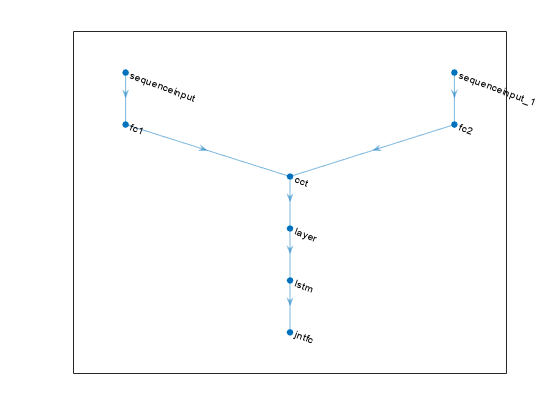
Create a deep neural network to be used as approximation model within the actor. The output layer must have three elements, each one expressing the value of executing the corresponding action, given the observation. To create a recurrent neural network, usesequenceInputLayer as the input layer and include anlstmLayer as one of the other network layers.
% Define paths inPath1 = [ sequenceInputLayer(prod(obsInfo(1).Dimension)) fullyConnectedLayer(prod(actInfo.Dimension),Name="fc1") ];
inPath2 = [ sequenceInputLayer(prod(obsInfo(2).Dimension)) fullyConnectedLayer(prod(actInfo.Dimension),Name="fc2") ];
% Concatenate previous paths outputs along first dimension jointPath = [ concatenationLayer(1,2,Name="cct") tanhLayer lstmLayer(8,OutputMode="sequence") fullyConnectedLayer( ... prod(numel(actInfo.Elements)), ... Name="jntfc") ];
% Assemble dlnetwork object net = dlnetwork; net = addLayers(net,inPath1); net = addLayers(net,inPath2); net = addLayers(net,jointPath);
% Connect layers net = connectLayers(net,"fc1","cct/in1"); net = connectLayers(net,"fc2","cct/in2");
% Plot network plot(net)
% initialize network and display the number of weights. net = initialize(net); summary(net)
Initialized: true
Number of learnables: 386
Inputs: 1 'sequenceinput' Sequence input with 4 dimensions 2 'sequenceinput_1' Sequence input with 1 dimensions
Since each element of the output layer must represent the probability of executing one of the possible actions the software automatically adds asoftmaxLayer as a final output layer if you do not specify it explicitly.
Create the actor with rlDiscreteCategoricalActor, using the network and the observations and action specification objects. When the network has multiple input layers, they are automatically associated with the environment observation channels according to the dimension specifications inobsInfo.
actor = rlDiscreteCategoricalActor(net, obsInfo, actInfo);
To return a vector of probabilities for each possible action, useevaluate.
[prob,state] = evaluate(actor, ... { rand(obsInfo(1).Dimension) , ... rand(obsInfo(2).Dimension) }); prob{1}
ans = 3x1 single column vector
0.3403
0.3114
0.3483
To return an action sampled from the distribution, usegetAction.
act = getAction(actor, ... { rand(obsInfo(1).Dimension) , ... rand(obsInfo(2).Dimension) }); act{1}
Set the option to accelerate the gradient computations.
actor = accelerate(actor,true);
Each array within a cell contains the gradient of the sum of the outputs with respect to a group of parameters.
grp_batch = gradient(actor,"output-parameters", ... { rand([obsInfo(1).Dimension 5 9]) , ... rand([obsInfo(2).Dimension 5 9])} )
grp_batch=9×1 cell array {[-3.1996e-09 -4.5687e-09 -4.4820e-09 -4.6439e-09]} {[ -1.1544e-08]} {[ -1.1321e-08]} {[ -2.8436e-08]} {32x2 single } {32x8 single } {32x1 single } { 3x8 single } { 3x1 single }
If you use a batch of inputs, the gradient uses the whole input sequence (in this case nine steps), and all the gradients with respect to the independent batch dimensions (in this case five) are added together. Therefore, the returned gradient always has the same size as the output from getLearnableParameters.
Input Arguments
useAcceleration — Option to use acceleration for gradient computations
false (default) | true
Option to use acceleration for gradient computations, specified as a logical value. When useAcceleration is true, the gradient computations are accelerated by optimizing and caching some inputs needed by the automatic-differentiation computation graph. For more information, see Deep Learning Function Acceleration for Custom Training Loops.
Output Arguments
newAppx — Actor or critic
approximator object
New actor or critic, returned as an approximator object with the same type asoldAppx but with the gradient acceleration option set touseAcceleration.
Version History
Introduced in R2022a
R2024a: accelerate is not recommended
accelerate is no longer recommended.
Instead of using accelerate to accelerate the gradient computation of a function approximator object, use dlaccelerate on your loss function. Then use dlfeval on theAcceleratedFunction object returned by dlaccelerate.
This workflow is shown in the following table.
| accelerate: Not Recommended | dlaccelerate: Recommended |
|---|---|
| actor = accelerate(actor,true); g = gradient(actor,@customLoss,u); g{1} where:function loss = customLoss(y,varargin) loss = sum(y{1}.^2); | f = dlaccelerate(@customLoss); g = dlfeval(@customLoss,actor,dlarray(u)); g{1}where:function g = customLoss(actor,u) y = evaluate(actor,u); loss = sum(y{1}.^2); g = dlgradient(loss,actor.Learnables); |
For more information, see also gradient is not recommended.
For more information on using dlarray objects for custom deep learning training loops, see dlfeval, AcceleratedFunction, dlaccelerate.
For an example, see Train Reinforcement Learning Policy Using Custom Training Loop and Custom Training Loop with Simulink Action Noise.
See Also
Functions
Objects
- AcceleratedFunction | rlValueFunction | rlQValueFunction | rlVectorQValueFunction | rlContinuousDeterministicActor | rlDiscreteCategoricalActor | rlContinuousGaussianActor | rlContinuousDeterministicTransitionFunction | rlContinuousGaussianTransitionFunction | rlContinuousDeterministicRewardFunction | rlContinuousGaussianRewardFunction | rlIsDoneFunction