gradient - (Not recommended) Evaluate gradient of function approximator object given
observation and action input data - MATLAB ([original](https://www.mathworks.com/help/reinforcement-learning/ref/rl.function.rlcontinuousdeterministicactor.gradient.html)) ([raw](?raw))(Not recommended) Evaluate gradient of function approximator object given observation and action input data
Since R2022a
Syntax
Description
[grad](#mw%5F69373c0f-c98b-4e35-a567-c80cb3ba60d6) = gradient([fcnAppx](#mw%5Fe9c66d2f-f484-41bc-8899-ae3caec9a948),'output-input',[inData](#mw%5Fb4650f92-4005-482d-a4f8-d5a5fef73dd6)) evaluates the gradient of the sum of the outputs of the function approximator objectfcnAppx with respect to its inputs. It returns the value of the gradient grad when the input of fcnAppx isinData.
[grad](#mw%5F69373c0f-c98b-4e35-a567-c80cb3ba60d6) = gradient([fcnAppx](#mw%5Fe9c66d2f-f484-41bc-8899-ae3caec9a948),'output-parameters',[inData](#mw%5Fb4650f92-4005-482d-a4f8-d5a5fef73dd6)) evaluates the gradient of the sum of the outputs of fcnAppx with respect to its parameters.
[grad](#mw%5F69373c0f-c98b-4e35-a567-c80cb3ba60d6) = gradient([fcnAppx](#mw%5Fe9c66d2f-f484-41bc-8899-ae3caec9a948),[lossFcn](#mw%5F3e73374f-5c83-490a-9a3b-bb272a78c290),[inData](#mw%5Fb4650f92-4005-482d-a4f8-d5a5fef73dd6),[fcnData](#mw%5F7fdcda92-fe2c-47ea-aad2-705ae0a6ca95)) evaluates the gradient of a loss function associated to the function handlelossFcn, with respect to the parameters offcnAppx. The last optional argument fcnData can contain additional inputs for the loss function.
Examples
Calculate Gradients for Continuous Gaussian Actor
Create observation and action specification objects (or alternatively use getObservationInfo andgetActionInfo to extract the specification objects from an environment). For this example, define an observation space with three channels. The first channel carries an observation from a continuous three-dimensional space, so that a single observation is a column vector containing three doubles. The second channel carries a discrete observation made of a two-dimensional row vector that can take one of five different values. The third channel carries a discrete scalar observation that can be either zero or one. Finally, the action space is a continuous four-dimensional space, so that a single action is a column vector containing four doubles, each between-10 and 10.
obsInfo = [ rlNumericSpec([3 1]) rlFiniteSetSpec({[1 2],[3 4],[5 6],[7 8],[9 10]}) rlFiniteSetSpec([0 1]) ];
actInfo = rlNumericSpec([4 1], ... UpperLimit= 10ones(4,1), ... LowerLimit=-10ones(4,1) );
To approximate the policy within the actor, use a recurrent deep neural network. For a continuous Gaussian actor, the network must have two output layers (one for the mean values the other for the standard deviation values), each having as many elements as the dimension of the action space.
Create a the network, defining each path as an array of layer objects. UsesequenceInputLayer as the input layer and include anlstmLayer as one of the other network layers. Also use a softplus layer to enforce nonnegativity of the standard deviations and a ReLU layer to scale the mean values to the desired output range. Get the dimensions of the observation and action spaces from the environment specification objects, and specify a name for the input layers, so you can later explicitly associate them with the appropriate environment channel.
obs1Path = [
sequenceInputLayer( ...
prod(obsInfo(1).Dimension), ...
Name="obs1InLyr")
fullyConnectedLayer(32,Name="obs1PthOutLyr")
];
obs2Path = [ sequenceInputLayer( ... prod(obsInfo(2).Dimension), ... Name="obs2InLyr") fullyConnectedLayer(32,Name="obs2PthOutLyr") ];
obs3Path = [ sequenceInputLayer( ... prod(obsInfo(3).Dimension), ... Name="obs3InLyr") fullyConnectedLayer(32,Name="obs3PthOutLyr") ];
% Concatenate inputs along the first available dimension comPath = [ concatenationLayer(1,3,Name="comPthInLyr") reluLayer lstmLayer(8,OutputMode="sequence",Name="lstm") fullyConnectedLayer(16) reluLayer(Name="comPthOutLyr") ];
% Path layers for mean value % Using tanhLayer & scalingLayer to scale range from (-1,1) to (-10,10) meanPath = [ fullyConnectedLayer(prod(actInfo(1).Dimension), ... Name="meanPthInLyr") tanhLayer scalingLayer(Name="meanOutLyr", ... Scale=actInfo(1).UpperLimit) ];
% Path layers for standard deviations % Using softplus layer to make them nonnegative stdPath = [ fullyConnectedLayer(prod(actInfo(1).Dimension), ... Name="stdPthInLyr") softplusLayer(Name="stdOutLyr") ];
% Assemble dlnetwork object. net = dlnetwork; net = addLayers(net,obs1Path); net = addLayers(net,obs2Path); net = addLayers(net,obs3Path); net = addLayers(net,comPath); net = addLayers(net,meanPath); net = addLayers(net,stdPath);
% Connect layers. net = connectLayers(net,"obs1PthOutLyr","comPthInLyr/in1"); net = connectLayers(net,"obs2PthOutLyr","comPthInLyr/in2"); net = connectLayers(net,"obs3PthOutLyr","comPthInLyr/in3"); net = connectLayers(net,"comPthOutLyr","meanPthInLyr/in"); net = connectLayers(net,"comPthOutLyr","stdPthInLyr/in");
% Plot network. plot(net)

% Initialize network. net = initialize(net);
% Display the number of learnable parameters. summary(net)
Initialized: true
Number of learnables: 3.9k
Inputs: 1 'obs1InLyr' Sequence input with 3 dimensions 2 'obs2InLyr' Sequence input with 2 dimensions 3 'obs3InLyr' Sequence input with 1 dimensions
Create the actor with rlContinuousGaussianActor, using the network, the observations and action specification objects, as well as the names of the network input layer and the options object.
actor = rlContinuousGaussianActor(net, obsInfo, actInfo, ... ActionMeanOutputNames="meanOutLyr",... ActionStandardDeviationOutputNames="stdOutLyr",... ObservationInputNames=["obs1InLyr","obs2InLyr","obs3InLyr"]);
To return mean value and standard deviations of the Gaussian distribution as a function of the current observation, use evaluate.
[prob,state] = evaluate(actor, {rand([obsInfo(1).Dimension 1 1]) , ... rand([obsInfo(2).Dimension 1 1]) , ... rand([obsInfo(3).Dimension 1 1]) });
The result is a cell array with two elements, the first one containing a vector of mean values, and the second containing a vector of standard deviations.
ans = 4×1 single column vector
0.0408
0.1472
-0.0644 -0.0433
ans = 4×1 single column vector
0.6966
0.6921
0.6795
0.6859
To return an action sampled from the distribution, usegetAction.
act = getAction(actor, {rand(obsInfo(1).Dimension) , ... rand(obsInfo(2).Dimension) , ... rand(obsInfo(3).Dimension) }); act{1}
ans = 4×1 single column vector
-0.0170 1.8817 0.4884 -0.4666
Calculate the gradients of the sum of the outputs (all the mean values plus all the standard deviations) with respect to the inputs, given a random observation.
gro = gradient(actor,"output-input", ... {rand(obsInfo(1).Dimension) , ... rand(obsInfo(2).Dimension) , ... rand(obsInfo(3).Dimension)} )
gro=3×1 cell array {3×1 single } {[-0.0424 0.0307]} {[ 0.0499]}
The result is a cell array with as many elements as the number of input channels. Each element contains the derivatives of the sum of the outputs with respect to each component of the input channel. Display the gradient with respect to the element of the second channel.
ans = 1×2 single row vector
-0.0424 0.0307
Obtain the gradient with respect of five independent sequences, each one made of nine sequential observations.
gro_batch = gradient(actor,"output-input", ... {rand([obsInfo(1).Dimension 5 9]) , ... rand([obsInfo(2).Dimension 5 9]) , ... rand([obsInfo(3).Dimension 5 9])} )
gro_batch=3×1 cell array {3×1×5×9 single} {1×2×5×9 single} {1×1×5×9 single}
Display the derivative of the sum of the outputs with respect to the third observation element of the first input channel, after the seventh sequential observation in the fourth independent batch.
Set the option to accelerate the gradient computations.
actor = accelerate(actor,true);
Calculate the gradients of the sum of the outputs with respect to the parameters, given a random observation.
grp = gradient(actor,"output-parameters", ... {rand(obsInfo(1).Dimension) , ... rand(obsInfo(2).Dimension) , ... rand(obsInfo(3).Dimension)} )
grp=15×1 cell array {32×3 single} {32×1 single} {32×2 single} {32×1 single} {32×1 single} {32×1 single} {32×96 single} {32×8 single} {32×1 single} {16×8 single} {16×1 single} { 4×16 single} { 4×1 single} { 4×16 single} { 4×1 single}
Each array within a cell contains the gradient of the sum of the outputs with respect to a group of parameters.
grp_batch = gradient(actor,"output-parameters", ... {rand([obsInfo(1).Dimension 5 9]) , ... rand([obsInfo(2).Dimension 5 9]) , ... rand([obsInfo(3).Dimension 5 9])} )
grp_batch=15×1 cell array {32×3 single} {32×1 single} {32×2 single} {32×1 single} {32×1 single} {32×1 single} {32×96 single} {32×8 single} {32×1 single} {16×8 single} {16×1 single} { 4×16 single} { 4×1 single} { 4×16 single} { 4×1 single}
If you use a batch of inputs, gradient uses the whole input sequence (in this case nine steps), and all the gradients with respect to the independent batch dimensions (in this case five) are added together. Therefore, the returned gradient has always the same size as the output from getLearnableParameters.
Calculate Gradients for Vector Q-Value Function
Create observation and action specification objects (or alternatively use getObservationInfo andgetActionInfo to extract the specification objects from an environment). For this example, define an observation space made of two channels. The first channel carries an observation from a continuous four-dimensional space. The second carries a discrete scalar observation that can be either zero or one. Finally, the action space consists of a scalar that can be -1,0, or 1.
obsInfo = [ rlNumericSpec([4 1]) rlFiniteSetSpec([0 1]) ];
actInfo = rlFiniteSetSpec([-1 0 1]);
To approximate the vector Q-value function within the critic, use a recurrent deep neural network. The output layer must have three elements, each one expressing the value of executing the corresponding action, given the observation.
Create the neural network, defining each network path as an array of layer objects. Get the dimensions of the observation and action spaces from the environment specification objects, use sequenceInputLayer as the input layer, and include an lstmLayer as one of the other network layers.
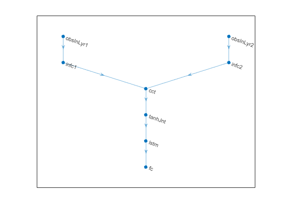
% First path inPath1 = [ sequenceInputLayer( ... prod(obsInfo(1).Dimension), ... Name="obsInLyr1") fullyConnectedLayer( ... prod(actInfo.Dimension), ... Name="infc1") ];
% Second path inPath2 = [ sequenceInputLayer( ... prod(obsInfo(2).Dimension), ... Name="obsInLyr2") fullyConnectedLayer( ... prod(actInfo.Dimension), ... Name="infc2") ];
% Concatenate inputs along first available dimension. jointPath = [ concatenationLayer(1,2,Name="cct") tanhLayer(Name="tanhJnt") lstmLayer(8,OutputMode="sequence") fullyConnectedLayer(prod(numel(actInfo.Elements))) ];
Assemble dlnetwork object and add layers.
net = dlnetwork; net = addLayers(net,inPath1); net = addLayers(net,inPath2); net = addLayers(net,jointPath);
Connect layers.
net = connectLayers(net,"infc1","cct/in1"); net = connectLayers(net,"infc2","cct/in2");
Plot network.
Initialize the network.
Display the number of weights.
Initialized: true
Number of learnables: 386
Inputs: 1 'obsInLyr1' Sequence input with 4 dimensions 2 'obsInLyr2' Sequence input with 1 dimensions
Create the critic with rlVectorQValueFunction, using the network and the observation and action specification objects.
critic = rlVectorQValueFunction(net,obsInfo,actInfo);
To return the value of the actions as a function of the current observation, usegetValue or evaluate.
val = evaluate(critic, ... {rand(obsInfo(1).Dimension), ... rand(obsInfo(2).Dimension)})
val = 1×1 cell array {3×1 single}
When you use evaluate, the result is a single-element cell array, containing a vector with the values of all the possible actions, given the observation.
ans = 3×1 single column vector
0.1293-0.0549 0.0425
Calculate the gradients of the sum of the outputs with respect to the inputs, given a random observation.
gro = gradient(critic,"output-input", ... {rand(obsInfo(1).Dimension) , ... rand(obsInfo(2).Dimension) } )
gro=2×1 cell array {4×1 single} {[ 0.0611]}
The result is a cell array with as many elements as the number of input channels. Each element contains the derivative of the sum of the outputs with respect to each component of the input channel. Display the gradient with respect to the element of the second channel.
Obtain the gradient with respect of five independent sequences each one made of nine sequential observations.
gro_batch = gradient(critic,"output-input", ... {rand([obsInfo(1).Dimension 5 9]) , ... rand([obsInfo(2).Dimension 5 9]) } )
gro_batch=2×1 cell array {4×1×5×9 single} {1×1×5×9 single}
Display the derivative of the sum of the outputs with respect to the third observation element of the first input channel, after the seventh sequential observation in the fourth independent batch.
Set the option to accelerate the gradient computations.
critic = accelerate(critic,true);
Calculate the gradients of the sum of the outputs with respect to the parameters, given a random observation.
grp = gradient(critic,"output-parameters", ... {rand(obsInfo(1).Dimension) , ... rand(obsInfo(2).Dimension) } )
grp=9×1 cell array {[-0.0178 -0.0052 -0.0588 -0.0114]} {[ -0.0597]} {[ 0.0873]} {[ 0.0962]} {32×2 single } {32×8 single } {32×1 single } { 3×8 single } { 3×1 single }
Each array within a cell contains the gradient of the sum of the outputs with respect to a group of parameters.
grp_batch = gradient(critic,"output-parameters", ... {rand([obsInfo(1).Dimension 5 9]) , ... rand([obsInfo(2).Dimension 5 9]) })
grp_batch=9×1 cell array {[-2.4487 -2.3282 -2.4941 -2.5877]} {[ -5.1411]} {[ 4.4295]} {[ 9.2137]} {32×2 single } {32×8 single } {32×1 single } { 3×8 single } { 3×1 single }
If you use a batch of inputs, gradient uses the whole input sequence (in this case nine steps), and all the gradients with respect to the independent batch dimensions (in this case five) are added together. Therefore, the returned gradient always has the same size as the output from getLearnableParameters.
Input Arguments
inData — Input data for the function approximator
cell array
Input data for the function approximator, specified as a cell array with as many elements as the number of input channels of fcnAppx. In the following section, the number of observation channels is indicated by_NO_.
- If
fcnAppxis anrlQValueFunction, anrlContinuousDeterministicTransitionFunctionor anrlContinuousGaussianTransitionFunctionobject, then each of the first NO elements ofinDatamust be a matrix representing the current observation from the corresponding observation channel. They must be followed by a final matrix representing the action. - If
fcnAppxis a function approximator object representing an actor or critic (but not anrlQValueFunctionobject),inDatamust contain_NO_ elements, each one being a matrix representing the current observation from the corresponding observation channel. - If
fcnAppxis anrlContinuousDeterministicRewardFunction, anrlContinuousGaussianRewardFunction, or anrlIsDoneFunctionobject, then each of the first_NO_ elements ofinDatamust be a matrix representing the current observation from the corresponding observation channel. They must be followed by a matrix representing the action, and finally by NO elements, each one being a matrix representing the next observation from the corresponding observation channel.
Each element of inData must be a matrix of dimension_MC_-by-_LB_-by-LS, where:
- MC corresponds to the dimensions of the associated input channel.
- LB is the batch size. To specify a single observation, set LB = 1. To specify a batch of (independent) observations, specify_LB_ > 1. If
inDatahas multiple elements, then LB must be the same for all elements ofinData. - LS specifies the sequence length (along the time dimension) for recurrent neural network. If
fcnAppxdoes not use a recurrent neural network, (which is the case of environment function approximators, as they do not support recurrent neural networks) then LS = 1. IfinDatahas multiple elements, then_LS_ must be the same for all elements ofinData.
For more information on input and output formats for recurrent neural networks, see the Algorithms section of lstmLayer.
Example: {rand(8,3,64,1),rand(4,1,64,1),rand(2,1,64,1)}
lossFcn — Loss function
function handle
Loss function, specified as a function handle to a user-defined function. The user defined function can either be an anonymous function or a function on the MATLAB path. The function first input parameter must be a cell array like the one returned from the evaluation of fcnAppx. For more information, see the description ofoutData in evaluate. The second, optional, input argument of lossFcn contains additional data that might be needed for the gradient calculation, as described below infcnData. For an example of the signature that this function must have, see Train Reinforcement Learning Policy Using Custom Training Loop.
Output Arguments
grad — Value of the gradient
cell array
Value of the gradient, returned as a cell array.
When the type of gradient is from the sum of the outputs with respect to the inputs of fcnAppx, then grad is a cell array in which each element contains the gradient of the sum of all the outputs with respect to the corresponding input channel.
The numerical array in each cell has dimensions_D_-by-_LB_-by-LS, where:
- D corresponds to the dimensions of the input channel of
fcnAppx. - LB is the batch size (length of a batch of independent inputs).
- LS is the sequence length (length of the sequence of inputs along the time dimension) for a recurrent neural network. If
fcnAppxdoes not use a recurrent neural network (which is the case of environment function approximators, as they do not support recurrent neural networks), then LS = 1.
When the type of gradient is from the output with respect to the parameters offcnAppx, then grad is a cell array in which each element contains the gradient of the sum of outputs belonging to an output channel with respect to the corresponding group of parameters. The gradient is calculated using the whole history of LS inputs, and all the_LB_ gradients with respect to the independent input sequences are added together in grad. Therefore,grad has always the same size as the result from getLearnableParameters.
For more information on input and output formats for recurrent neural networks, see the Algorithms section of lstmLayer.
Version History
Introduced in R2022a
R2024a: gradient is not recommended
gradient is no longer recommended.
Instead of using gradient on a function approximator object, write an appropriate loss function that takes as arguments both the approximation object and its input. In the loss function you typically use evaluate to calculate the output and dlgradient to calculate the gradient. Then call dlfeval, supplying both the approximator object and it inputs as arguments.
This workflow is shown in the following table.
| gradient: Not Recommended | dlfeval and dlgradient: Recommended |
|---|---|
| g = gradient(actor,"output-input",u); g{1} | g = dlfeval(@myOIGFcn,actor,dlarray(u)); g{1}where:function g = myOIGFcn(actor,u) y = evaluate(actor,u); loss = sum(y{1}); g = dlgradient(loss,u); |
| g = gradient(actor,"output-parameters",u); g{1} | g = dlfeval(@myOPGFcn,actor,dlarray(u)); g{1}where:function g = myOIGFcn(actor,u) y = evaluate(actor,u); loss = sum(y{1}); g = dlgradient(loss,actor.Learnables); |
| g = gradient(actor,@customLoss23b,u); g{1} where:function loss = customLoss23b(y,varargin) loss = sum(y{1}.^2); | g = dlfeval(@customLoss24a,actor,dlarray(u)); g{1}where:function g = customLoss24a(actor,u) y = evaluate(actor,u); loss = sum(y{1}.^2); g = dlgradient(loss,actor.Learnables); |
For more information, see also accelerate is not recommended.
For more information on using dlarray objects for custom deep learning training loops, see dlfeval, AcceleratedFunction, dlaccelerate.
For an example, see Train Reinforcement Learning Policy Using Custom Training Loop and Custom Training Loop with Simulink Action Noise.
See Also
Functions
Objects
- AcceleratedFunction | rlValueFunction | rlQValueFunction | rlVectorQValueFunction | rlContinuousDeterministicActor | rlDiscreteCategoricalActor | rlContinuousGaussianActor | rlContinuousDeterministicTransitionFunction | rlContinuousGaussianTransitionFunction | rlContinuousDeterministicRewardFunction | rlContinuousGaussianRewardFunction | rlIsDoneFunction