predict - Predict next observation, next reward, or episode termination given observation and
action input data - MATLAB ([original](https://www.mathworks.com/help/reinforcement-learning/ref/rl.function.rlcontinuousdeterministictransitionfunction.predict.html)) ([raw](?raw))Predict next observation, next reward, or episode termination given observation and action input data
Since R2022a
Syntax
Description
[predNextObs](#mw%5Ffbb14362-8b6d-4588-be0f-a092ddb9d7d4) = predict([tsnFcnAppx](#mw%5F1302314a-ddc6-49cc-8797-30ef6f6ee3ef),[obs](#mw%5Ff3d8a0a9-4cb3-4e08-995d-3f3fcc677362),[act](#mw%5F34aa0aa3-4dd0-496d-882e-69e1dbc49339)) evaluates the environment transition function approximator objecttsnFcnAppx and returns the predicted next observationnextObs, given the current observation obs and the action act.
[predReward](#mw%5F3655a1a5-b23b-4bfc-87ee-12c27fadec19) = predict([rwdFcnAppx](#mw%5F576e8fa4-a3b0-4396-99f0-563cd18c82b0),[obs](#mw%5Ff3d8a0a9-4cb3-4e08-995d-3f3fcc677362),[act](#mw%5F34aa0aa3-4dd0-496d-882e-69e1dbc49339),[nextObs](#mw%5F9a4def93-3825-4618-bfc9-343d2eea789a)) evaluates the environment reward function approximator objectrwdFcnAppx and returns the predicted rewardpredReward, given the current observation obs, the action act, and the next observationnextObs.
[predIsDone](#mw%5F038c579a-0383-4c71-9deb-49a41101b8f1) = predict([idnFcnAppx](#mw%5F41dce91d-f29c-4cc2-94af-5730a4f0d515),[obs](#mw%5Ff3d8a0a9-4cb3-4e08-995d-3f3fcc677362),[act](#mw%5F34aa0aa3-4dd0-496d-882e-69e1dbc49339)) evaluates the environment is-done function approximator objectidnFcnAppx and returns the predicted is-done statuspredIsDone, given the current observation obs, the action act, and the next observationnextObs.
___ = predict(___,UseForward=[useForward](#mw%5Fd5adc863-c226-4bde-bb2a-c3bcea401aaa%5Fsep%5Fmw%5F7f8a74e4-f9cb-4418-bfe7-55c39bddd077)) allows you to explicitly call a forward pass when computing gradients.
Examples
Create observation and action specification objects (or alternatively use getObservationInfo and getActionInfo to extract the specification objects from an environment). For this example, two observation channels carry vectors in a four- and two-dimensional space, respectively. The action is a continuous three-dimensional vector.
obsInfo = [ rlNumericSpec([4 1],UpperLimit=10ones(4,1)); rlNumericSpec([1 2],UpperLimit=20ones(1,2)) ];
actInfo = rlNumericSpec([3 1]);
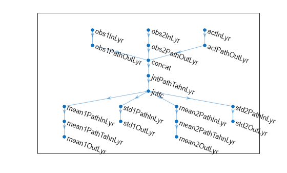
Create a deep neural network to use as approximation model for the transition function approximator. For a continuous Gaussian transition function approximator, the network must have two output layers for each observation (one for the mean values the other for the standard deviation values).
Define each network path as an array of layer objects. Get the dimensions of the observation and action spaces from the environment specification objects, and specify a name for the input layers, so you can later explicitly associate them with the appropriate environment channel.
% Input path layers from first observation channel obs1Path = [ featureInputLayer( ... prod(obsInfo(1).Dimension), ... Name="obs1InLyr") fullyConnectedLayer(5,Name="obs1PathOutLyr") ];
% Input path layers from second observation channel obs2Path = [ featureInputLayer( ... prod(obsInfo(2).Dimension), ... Name="obs2InLyr") fullyConnectedLayer(5,Name="obs2PathOutLyr") ];
% Input path layers from action channel actPath = [ featureInputLayer( ... prod(actInfo(1).Dimension), ... Name="actInLyr") fullyConnectedLayer(5,Name="actPathOutLyr") ];
% Joint path layers, concatenate 3 inputs along first dimension jointPath = [ concatenationLayer(1,3,Name="concat") tanhLayer(Name="jntPathTahnLyr"); fullyConnectedLayer(10,Name="jntfc") ];
% Path layers for mean values of first predicted obs % Using tanh and scaling layers to scale range from (-1,1) to (-10,10) % Note that scale vector must be a column vector mean1Path = [ fullyConnectedLayer(prod(obsInfo(1).Dimension), ... Name="mean1PathInLyr"); tanhLayer(Name="mean1PathTahnLyr"); scalingLayer(Name="mean1OutLyr", ... Scale=obsInfo(1).UpperLimit) ];
% Path layers for standard deviations first predicted obs % Using softplus layer to make them non negative std1Path = [ fullyConnectedLayer(prod(obsInfo(1).Dimension), ... Name="std1PathInLyr"); softplusLayer(Name="std1OutLyr") ];
% Path layers for mean values of second predicted obs % Using tanh and scaling layers to scale range from (-1,1) to (-20,20) % Note that scale vector must be a column vector mean2Path = [ fullyConnectedLayer(prod(obsInfo(2).Dimension), ... Name="mean2PathInLyr"); tanhLayer(Name="mean2PathTahnLyr"); scalingLayer(Name="mean2OutLyr", ... Scale=obsInfo(2).UpperLimit(:)) ];
% Path layers for standard deviations second predicted obs % Using softplus layer to make them non negative std2Path = [ fullyConnectedLayer(prod(obsInfo(2).Dimension), ... Name="std2PathInLyr"); softplusLayer(Name="std2OutLyr") ];
% Assemble dlnetwork object. net = dlnetwork; net = addLayers(net,obs1Path); net = addLayers(net,obs2Path); net = addLayers(net,actPath); net = addLayers(net,jointPath); net = addLayers(net,mean1Path); net = addLayers(net,std1Path); net = addLayers(net,mean2Path); net = addLayers(net,std2Path);
% Connect layers. net = connectLayers(net,"obs1PathOutLyr","concat/in1"); net = connectLayers(net,"obs2PathOutLyr","concat/in2"); net = connectLayers(net,"actPathOutLyr","concat/in3"); net = connectLayers(net,"jntfc","mean1PathInLyr/in"); net = connectLayers(net,"jntfc","std1PathInLyr/in"); net = connectLayers(net,"jntfc","mean2PathInLyr/in"); net = connectLayers(net,"jntfc","std2PathInLyr/in");
% Plot network. plot(net)
% Initialize network. net = initialize(net);
% Display the number of weights. summary(net)
Initialized: true
Number of learnables: 352
Inputs: 1 'obs1InLyr' 4 features 2 'obs2InLyr' 2 features 3 'actInLyr' 3 features
Create a continuous Gaussian transition function approximator object, specifying the names of all the input and output layers.
tsnFcnAppx = rlContinuousGaussianTransitionFunction(... net,obsInfo,actInfo,... ObservationInputNames=["obs1InLyr","obs2InLyr"], ... ActionInputNames="actInLyr", ... NextObservationMeanOutputNames= ... ["mean1OutLyr","mean2OutLyr"], ... NextObservationStandardDeviationOutputNames= ... ["std1OutLyr","std2OutLyr"] );
Predict the next observation for a random observation and action.
predObs = predict(tsnFcnAppx, ... {rand(obsInfo(1).Dimension),rand(obsInfo(2).Dimension)}, ... {rand(actInfo(1).Dimension)})
predObs=1×2 cell array {4×1 single} {[-19.2685 -1.1779]}
Each element of the resulting cell array represents the prediction for the corresponding observation channel.
To display the mean values and standard deviations of the Gaussian probability distribution for the predicted observations, use evaluate.
predDst = evaluate(tsnFcnAppx, ... {rand(obsInfo(1).Dimension), ... rand(obsInfo(2).Dimension), ... rand(actInfo(1).Dimension)})
predDst=1×4 cell array {4×1 single} {[-16.6873 4.4006]} {4×1 single} {[0.7455 1.4318]}
The result is a cell array in which the first and second element represent the mean values for the predicted observations in the first and second channel, respectively. The third and fourth element represent the standard deviations for the predicted observations in the first and second channel, respectively.
Create an environment object and extract observation and action specifications. Alternatively, you can create specifications using rlNumericSpec and rlFiniteSetSpec.
env = rlPredefinedEnv("CartPole-Continuous"); obsInfo = getObservationInfo(env); actInfo = getActionInfo(env);
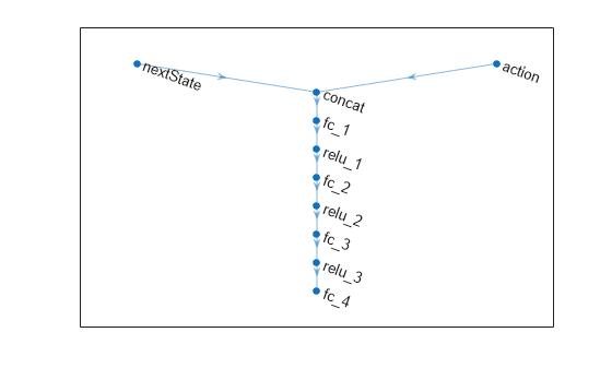
To approximate the reward function, create a deep neural network. For this example, the network has two input layers, one for the current action and one for the next observations. The single output layer contains a scalar, which represents the value of the predicted reward.
Define each network path as an array of layer objects. Get the dimensions of the observation and action spaces from the environment specifications, and specify a name for the input layers, so you can later explicitly associate them with the appropriate environment channel.
actionPath = featureInputLayer( ... actInfo.Dimension(1), ... Name="action");
nextStatePath = featureInputLayer( ... obsInfo.Dimension(1), ... Name="nextState");
commonPath = [concatenationLayer(1,2,Name="concat") fullyConnectedLayer(64) reluLayer fullyConnectedLayer(64) reluLayer fullyConnectedLayer(64) reluLayer fullyConnectedLayer(1)];
Assemble dlnetwork object.
net = dlnetwork(); net = addLayers(net,nextStatePath); net = addLayers(net,actionPath); net = addLayers(net,commonPath);
Connect layers.
net = connectLayers(net,"nextState","concat/in1"); net = connectLayers(net,"action","concat/in2");
Plot network.
Initialize network and display the number of weights.
net = initialize(net); summary(net)
Initialized: true
Number of learnables: 8.7k
Inputs: 1 'nextState' 4 features 2 'action' 1 features
Create a deterministic transition function object.
rwdFcnAppx = rlContinuousDeterministicRewardFunction(... net,obsInfo,actInfo,... ActionInputNames="action", ... NextObservationInputNames="nextState");
Using this reward function object, you can predict the next reward value based on the current action and next observation. For example, predict the reward for a random action and next observation. Since, for this example, only the action and the next observation influence the reward, use an empty cell array for the current observation.
act = rand(actInfo.Dimension); nxtobs = rand(obsInfo.Dimension); reward = predict(rwdFcnAppx, {}, {act}, {nxtobs})
To predict the reward, you can also use evaluate.
reward_ev = evaluate(rwdFcnAppx, {act,nxtobs} )
reward_ev = 1×1 cell array {[0.1034]}
Create an environment object and extract observation and action specifications. Alternatively, you can create specifications using rlNumericSpec and rlFiniteSetSpec.
env = rlPredefinedEnv("CartPole-Continuous"); obsInfo = getObservationInfo(env); actInfo = getActionInfo(env);
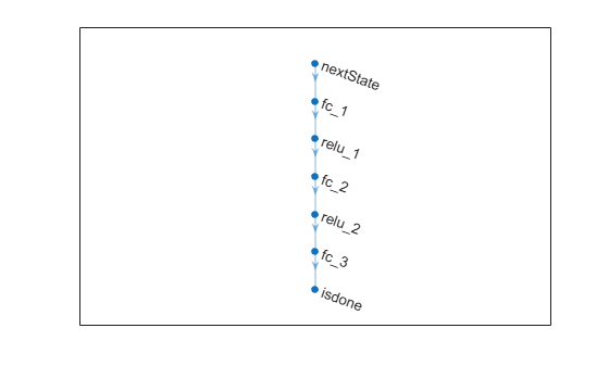
To approximate the is-done function, use a deep neural network. The network has one input channel for the next observations. The single output channel is for the predicted termination signal.
Create the neural network as a vector of layer objects.
net = [ featureInputLayer( ... obsInfo.Dimension(1), ... Name="nextState") fullyConnectedLayer(64) reluLayer fullyConnectedLayer(64) reluLayer fullyConnectedLayer(2) softmaxLayer(Name="isdone") ];
Convert to dlnetwork object.
Plot network.
Initialize network and display the number of weights.
net = initialize(net); summary(net);
Initialized: true
Number of learnables: 4.6k
Inputs: 1 'nextState' 4 features
Create an is-done function approximator object.
isDoneFcnAppx = rlIsDoneFunction(... net,obsInfo,actInfo,... NextObservationInputNames="nextState");
Using this is-done function approximator object, you can predict the termination signal based on the next observation. For example, predict the termination signal for a random next observation. Since for this example the termination signal only depends on the next observation, use empty cell arrays for the current action and observation inputs.
nxtobs = rand(obsInfo.Dimension); predIsDone = predict(isDoneFcnAppx,{},{},{nxtobs})
You can obtain the termination probability using evaluate.
predIsDoneProb = evaluate(isDoneFcnAppx,{nxtobs})
predIsDoneProb = 1×1 cell array {2×1 single}
ans = 2×1 single column vector
0.5405
0.4595
The first number is the probability of obtaining a 0 (no termination predicted), the second one is the probability of obtaining a 1 (termination predicted).
Input Arguments
Environment is-done function approximator object, specified as an rlIsDoneFunction object.
Observations, specified as a cell array with as many elements as there are observation input channels. Each element of obs contains an array of observations for a single observation input channel.
The dimensions of each element in obs are_MO_-by-LB, where:
- MO corresponds to the dimensions of the associated observation input channel.
- LB is the batch size. To specify a single observation, set LB = 1. To specify a batch of observations, specify LB > 1. If
valueReporqValueRephas multiple observation input channels, then LB must be the same for all elements ofobs.
LB must be the same for bothact and obs.
For more information on input and output formats for recurrent neural networks, see the Algorithms section of lstmLayer.
Action, specified as a single-element cell array that contains an array of action values.
The dimensions of this array are_MA_-by-LB, where:
- MA corresponds to the dimensions of the associated action specification.
- LB is the batch size. To specify a single observation, set LB = 1. To specify a batch of observations, specify LB > 1.
LB must be the same for bothact and obs.
For more information on input and output formats for recurrent neural networks, see the Algorithms section of lstmLayer.
Next observations, that is the observation following the actionact from the observation obs, specified as a cell array of the same dimension as obs.
Option to use forward pass, specified as a logical value. When you specifyUseForward=true the function calculates its outputs usingforward instead of predict. This allows layers such as batch normalization and dropout to appropriately change their behavior for training.
Example: true
Output Arguments
Predicted next observation, that is the observation predicted by the transition function approximator tsnFcnAppx given the current observationobs and the action act, returned as a cell array of the same dimension as obs.
Predicted reward, that is the reward predicted by the reward function approximatorrwdFcnAppx given the current observationobs, the action act, and the following observation nextObs, returned as asingle.
Predicted is-done episode status, that is the episode termination status predicted by the is-done function approximator rwdFcnAppx given the current observation obs, the action act, and the following observation nextObs, returned as adouble.
Note
If fcnAppx is an rlContinuousDeterministicRewardFunction object, thenevaluate behaves identically to predict except that it returns results inside a single-cell array. If fcnAppx is an rlContinuousDeterministicTransitionFunction object, thenevaluate behaves identically to predict. IffcnAppx is an rlContinuousGaussianTransitionFunction object, thenevaluate returns the mean value and standard deviation the observation probability distribution, while predict returns an observation sampled from this distribution. Similarly, for an rlContinuousGaussianRewardFunction object, evaluate returns the mean value and standard deviation the reward probability distribution, while predict returns a reward sampled from this distribution. Finally, if fcnAppx is anrlIsDoneFunction object, then evaluate returns the probabilities of the termination status being false or true, respectively, while predict returns a predicted termination status sampled with these probabilities.
Version History
Introduced in R2022a
See Also
Functions
- evaluate | runEpisode | update | rlOptimizer | syncParameters | getValue | getAction | getMaxQValue | getLearnableParameters | setLearnableParameters