How to Perform Data Analysis in Excel (original) (raw)
Last Updated : 10 Feb, 2026
Excel is one of the most used tools for data analysis, helping beginners easily clean organize, analyze and visualize data. It allows users to work with large datasets and extract meaningful insights without requiring advanced technical skills.
- Preparing and cleaning data for accurate analysis in Excel
- Applying key data analysis techniques such as sorting, filtering and visualization
- Using essential Excel tools and functions for effective decision-making
Preparing Data for Analysis
Before starting any analysis, your data must be accurate and well-structured. Poor data quality leads to incorrect insights.
**Data preparation in Excel includes:
- Removing duplicates and inconsistencies
- Handling unnecessary spaces and special characters
- Structuring data for easier analysis
Excel Tables and PivotTables make this process intuitive and efficient.
**How to Clean Data in Excel
**Remove Duplicates: Use Data -> Remove Duplicates to eliminate repeated records and ensure data accuracy.
**Use TRIM and CLEAN Functions
- TRIM removes extra spaces from text
- CLEAN removes non-printable characters
These functions are especially useful when data is imported from external sources.
**Sort and Structure Data: Convert your dataset into an Excel Table using Insert -> Table. Tables make sorting, filtering and analysis faster and more reliable.
Basic Methods of Data Analysis in Excel
Excel offers several methods to analyze data effectively. Here are some key techniques:
1. Charts and Visualization
Data Analysis Excel offers several different chart types available for you to choose from or you can use the Excel Recommended Charts option to look at charts specifically made for your data and choose one of those. Charts help you understand trends, patterns and relationships in data visually.
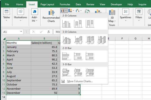
**Steps to Create a Chart
- Select your dataset
- Go to Insert -> Charts
- Choose a chart type such as Bar, Line or Pie
- Customize labels, titles and colors for clarity
Excel also provides Recommended Charts, which automatically suggest suitable visualizations.
**Preview Chart:
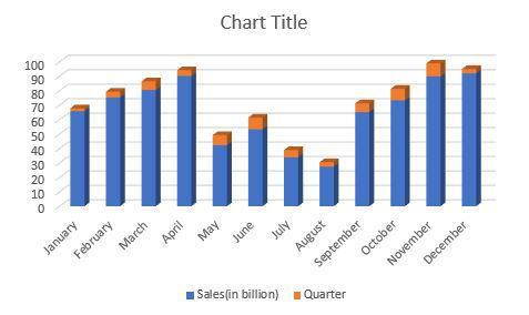
Bar Graph
2. Conditional Formatting
Conditional formatting helps highlight important patterns and trends in data by automatically applying colors or styles based on cell values. It allows users to quickly identify values that meet specific conditions without manually checking the dataset. In Excel, conditional formatting can be applied to a range of cells, an Excel table or a PivotTable. Follow the below steps:
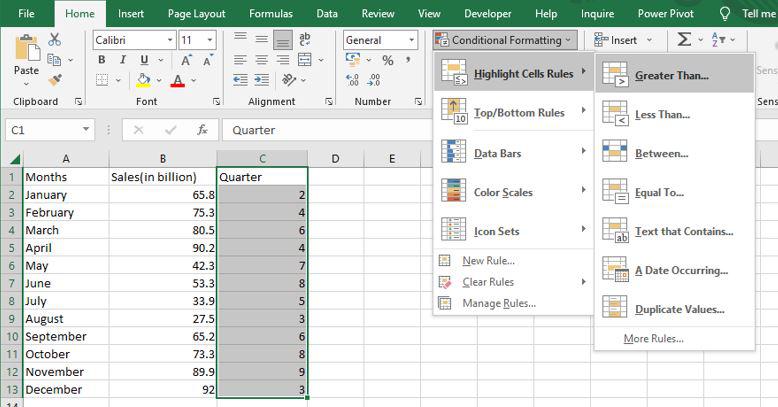
**Step 1: Go to Home > Conditional Formatting
Select any column from the table. Here we are going to select a Quarter column. After that go to the home tab on the top of the ribbon and then in the styles group select conditional formatting and then in the highlight cells rule select Greater than an option.
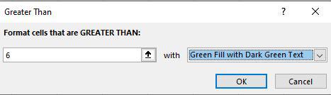
Then a greater than dialog box appears. Here first write the quarter value and then select the color.
**Step 2: Preview Result
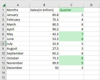
As you can see in the excel table Quarter column change the color of the values that are greater than 6.
3. Sorting Data
Sorting organizes data in a meaningful order, making it easier to analyze and compare values. In Excel, data can be sorted alphabetically, numerically, by date or even by cell color or icons. Sorting helps users quickly locate important information and understand data distribution.
- **Single-column sorting: Sort data in ascending or descending order
- **Multi-column sorting: Apply multiple sorting levels using different columns
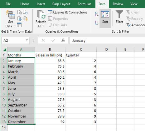
**Step 1: Select Data > Data Tab > Sort
Select any column from the table. Here we are going to select a Months column. After that go to the data tab on the top of the ribbon and then in the sort and filters group select sort.
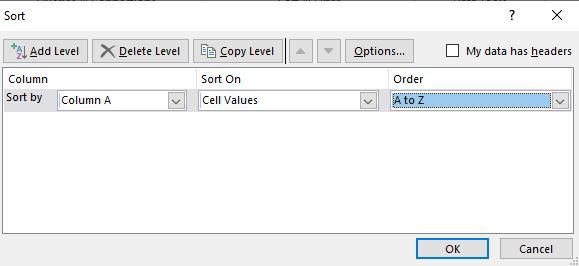
**Step 2: Select the Order
Then a sort dialog box appears. Here first select the column, then select sort on and then Order. After that click OK.
**Step 3: Preview Results
Now as you can see the months column is now arranged alphabetically.
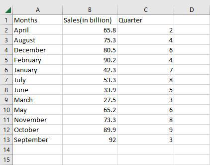
4. Filtering Data
Filtering allows you to display only the records that meet specific criteria while hiding the rest of the data. This makes it easier to focus on relevant information, especially when working with large datasets.
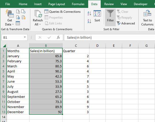
**Step 1: Select your dataset and go to Data > Filter
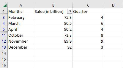
Select any column from the table. Here we are going to select a Sales column. After that go to the data tab on the top of the ribbon and then in the sort and filters group select filter.
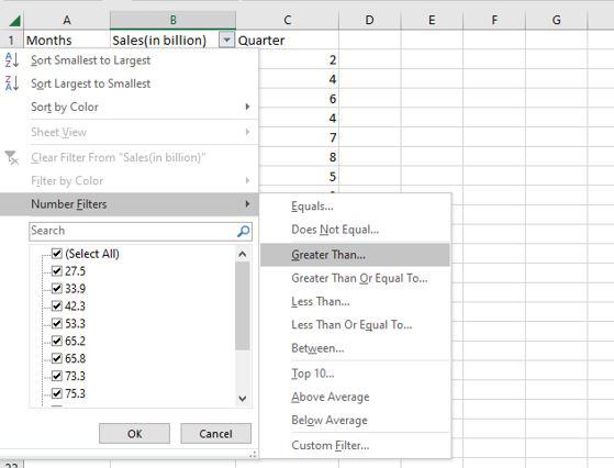
**Step 2: Select the Filter Option
The values in the sales column are then shown in a drop-down box. Here we are going to select a number of filters and then greater than.
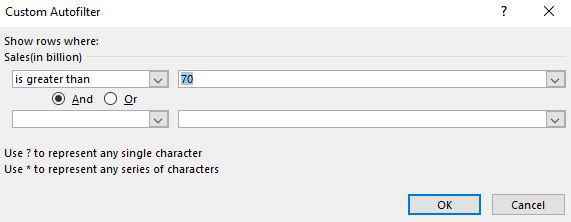
**Step 3: Select the Options
Then a custom auto filler dialog box appears. Here we are going to apply sales greater than 70 and then click OK.
**Step 4: Preview Results
Now as you can see only the rows greater than 70 are shown.
Excel offers several advanced tools to make data analysis more efficient and powerful. Here are some key tools you can use:
1. Power Query
- Automates data preparation by importing, transforming and combining data from multiple sources.
- **Example: Clean and merge datasets to create a unified report.
2. Data Analysis ToolPak
- Provides advanced statistical analysis tools like regression and ANOVA.
- **Example: Use regression to identify relationships between variables or ANOVA to analyze variance across groups.
3. Solver
- Optimizes complex problems by finding the best solution based on constraints.
- **Example: Minimize inventory costs while meeting demand by adjusting stock levels.
These tools help enhance Excel's capabilities for advanced data analysis, making it suitable for more sophisticated tasks.
Essential Excel Functions for Data Analysis
Excel’s built-in functions allow for quick calculations and summaries:
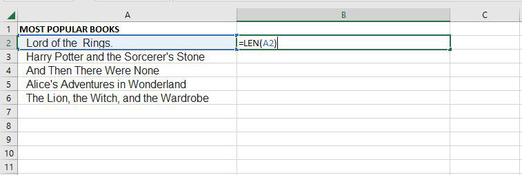
LEN
=LEN returns the number of characters in a text cell. Useful for identifying differences in product codes or IDs.
=LEN(Select Cell)
**Step 1: Use the LENGTH Function
To find the length of the text in cell A2, use the LENGTH function. This function calculates the number of characters in the given cell.
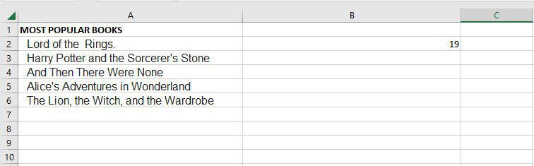
**Step 2: View the Length of Cell A2
Once you apply the LENGTH function, it will display the number of characters present in cell A2.
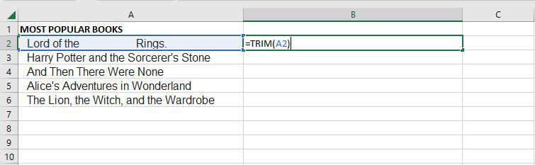
TRIM
=TRIM Removes extra spaces except single spaces between words.
=TRIM(Select Cell)
**Step 1: Use the TRIM Function
To remove all spaces from cell A2, apply the TRIM function.
**Step 2: Observe the Result
After using the TRIM function, all extra spaces will be removed from the text in cell A2.
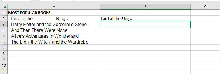
UPPER
Excel Text function "UPPER Function" will change the text to all capital letters (UPPERCASE). As a result, the function changes all of the characters in a text string input to upper case.
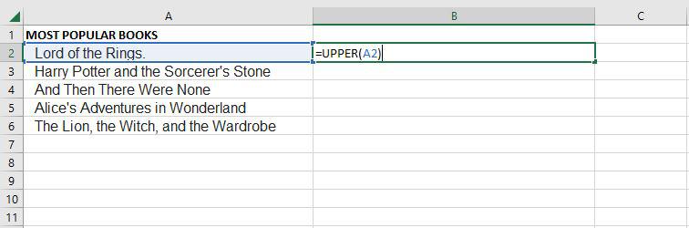
=UPPER(Text)
**Text (mandatory parameter): This is the text that we wish to change to uppercase. Text can relate to a cell or be a text string.
**Step 1: Use the UPPER Function
To convert the text in cell A2 to uppercase, use the UPPER function. This function transforms all lowercase letters into uppercase.
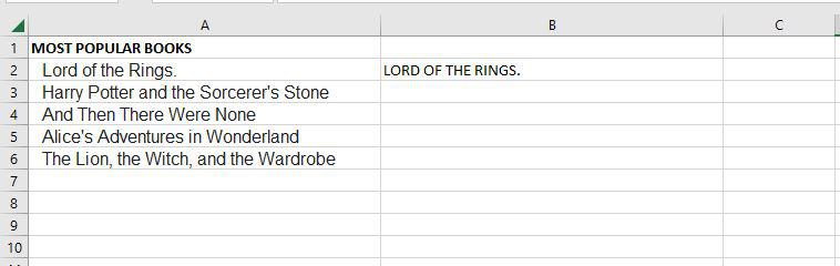
**Step 2: View the Converted Text
After applying the UPPER function, the text in cell A2 will be converted to uppercase.
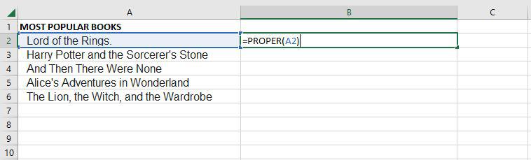
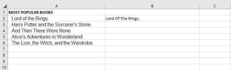
PROPER
Under Excel Text functions, the PROPER Function is listed. Any subsequent letters of text that come after a character other than a letter will also be capitalized by PROPER.
=PROPER(Text)
**Text (mandatory parameter): A formula that returns text, a cell reference or text in quote marks must surround the text you wish to partly capitalize.
**Step 1: Use the PROPER Function
To convert the text in cell A2 to proper case (where the first letter of each word is capitalized), use the PROPER function.
**Step 2: View the Converted Text
After applying the PROPER function, the text in cell A2 will be formatted with proper case, capitalizing the first letter of each word.
The PROPER function changes the initial letter of every word, letters that follow digits and other punctuation to uppercase. It could be where we least expect it. The characters for numbers and punctuation remain unaffected.
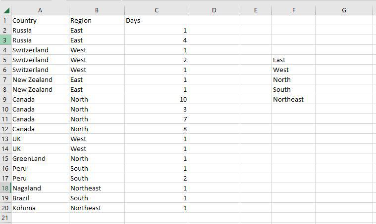
COUNTIF
Excel has a built-in function called COUNTIF that counts the given cells. The COUNTIF function can be used in both straightforward and sophisticated applications in data analysis excel. The fundamental application of counting particular numbers and words is covered in this.
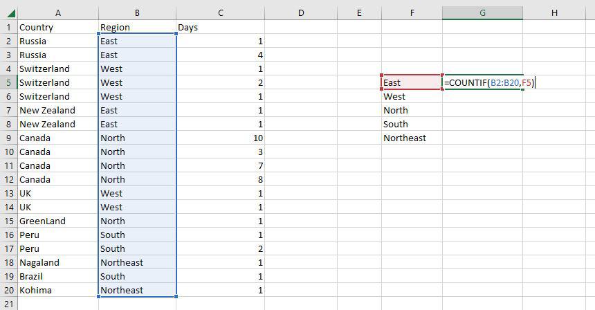
=COUNTIF(range,criteria)
- **Range: The size of the cell range to count.
- **Criteria: The standards by which cells are selected for counting.
**Step 1: Use the COUNTIF Function on the Range B2:B20
To count the number of regions of each type, apply the COUNTIF function to the range B2:B20.
**Step 2: Count the Different Regions in the Range F5:F9
Next, use the COUNTIF function on the range F5:F9 to count the different types of regions.
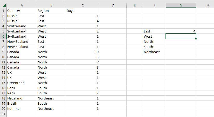
**Step 3: Verify the Count for Each Region
As you can see, the COUNTIF function has correctly enumerated the number of regions, such as the 4 East Regions, as expected.
AVERAGEIF
An Excel built-in function called AVERAGEIF determines the average of a range depending on a true or false condition.
=AVERAGEIF(range, criteria, [average_range])
- **Range: The size of the cell range to count.
- **Criteria: The standards by which cells are selected for counting.
- **Average Range: The range in which the function computes the average is known as the average range. But the average range is not required.
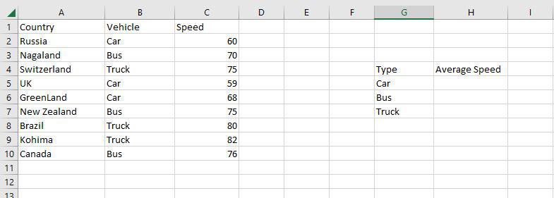
**Step 1: Use the AVERAGEIF Function on the Range B2:B10
To calculate the average speed of vehicles, apply the AVERAGEIF function on the range B2:B10.
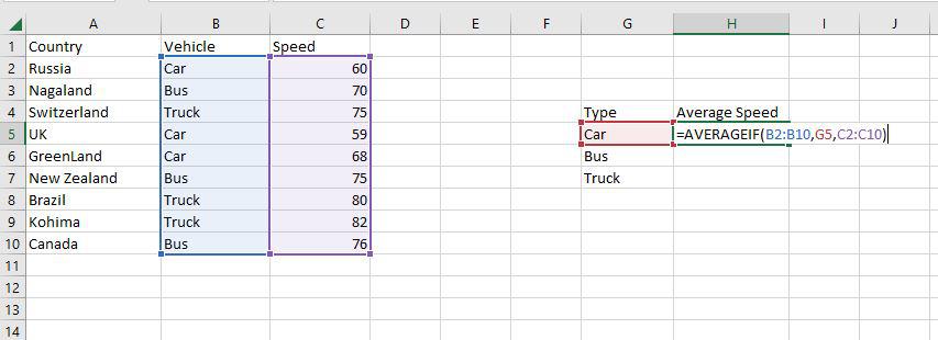
**Step 2: Use the AVERAGEIF Function on the Range H4:H7
Next, use the AVERAGEIF function on the range H4:H7 to find the average for the vehicles listed in that range.
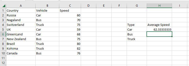
**Step 3: Verify the Average Calculation
As you can see, the AVERAGEIF function has correctly calculated the average speed of the vehicles, such as the 62.333 average for cars.
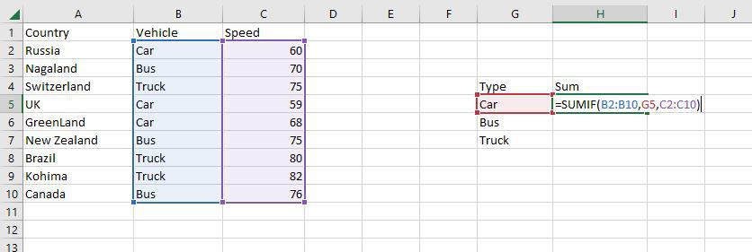
SUMIF
A built-in Excel function called SUMIF determines if a condition is true or false before adding the values in a range.
=SUMIF(range, criteria, [sum_range])
- **Range: The size of the cell range to count.
- **Criteria: The standards by which cells are selected for counting.
- **Sum Range: The range that the function uses to calculate the total is known as the sum range.
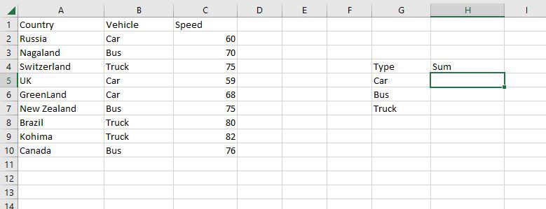
**Step 1: Use the SUMIF Function on the Range B2:B10
To calculate the sum of the vehicle's speed, apply the SUMIF function on the range B2:B10.
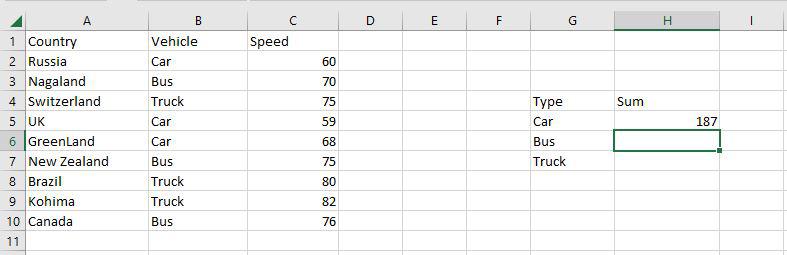
**Step 2: Use the SUMIF Function on the Range H4:H7
Next, use the SUMIF function on the range H4:H7 to find the sum of the vehicle speeds listed in that range.
**Step 3: Verify the Sum Calculation
As you can see, the SUMIF function has correctly calculated the total speed, such as the 187 sum for cars.
VLOOKUP
VLOOKUP is a built-in Excel function that permits searching across several columns.
=VLOOKUP(lookup_value, table_array, col_index_num, [range_lookup])
- **Lookup_value: Choose the cell that will be used to input the search criteria.
- **Table_array: The whole table range, which includes each and every cell.
- **Col_index_num: The information being searched for. The column's number, starting from the left, is the input.
- **Range_lookup: FALSE if text (0), TRUE if numbers (1).
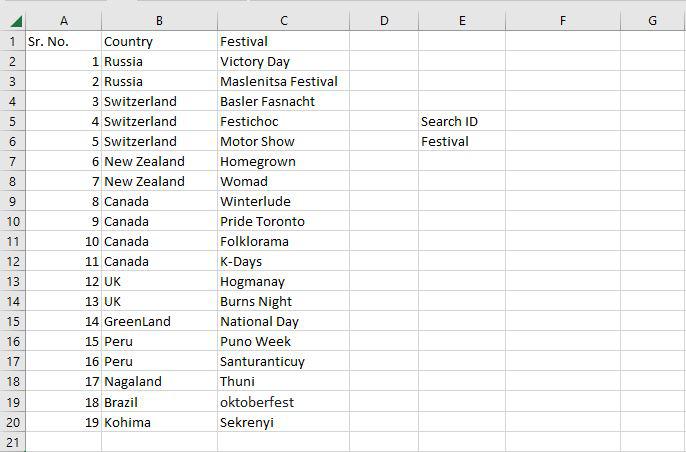
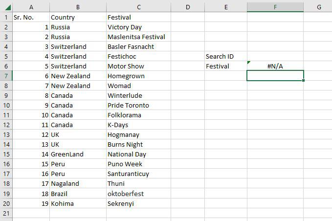
**Step 1: Use the VLOOKUP Function to Locate Festival Names
To locate the festival names based on their search ID, use the VLOOKUP function. The festival names will be determined by their corresponding search ID.
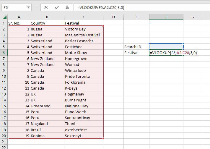
**Step 2: Set Up the VLOOKUP Function
In cell F5, enter the search query (lookup value). The table array range is A2:C20, with the col index number set to 3 (since the information is in the third column from the left). Set the range lookup to 0 (False) to ensure an exact match.
**Step 3: Handle the #N/A Value
If the lookup value in F5 does not exist in the table, the VLOOKUP function will return a #N/A value, indicating that no match was found.
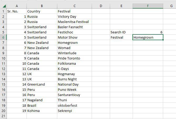
**Step 4: Locate the Festival Using VLOOKUP
The VLOOKUP function successfully identifies the Homegrown Festival with Search ID 6.
Pivot Table
In order to create the required report, a pivot table is a statistics tool that condenses and reorganizes specific columns and rows of data in a spreadsheet or database table. The utility simply "pivots" or rotates the data to examine it from various angles rather than altering the spreadsheet or database itself.
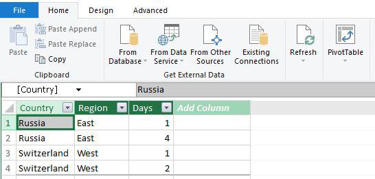
**Step 1: Select a Cell and Create a Pivot Table
Select any cell in your worksheet, go to the Home tab and click on "Pivot Table."
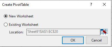
**Step 2: Choose the Pivot Table Location
In the Create Pivot Table dialog box, select "New Worksheet" and then click OK.
**Step 3: View the Created Pivot Table
You will now see a new worksheet with a blank Pivot Table created.
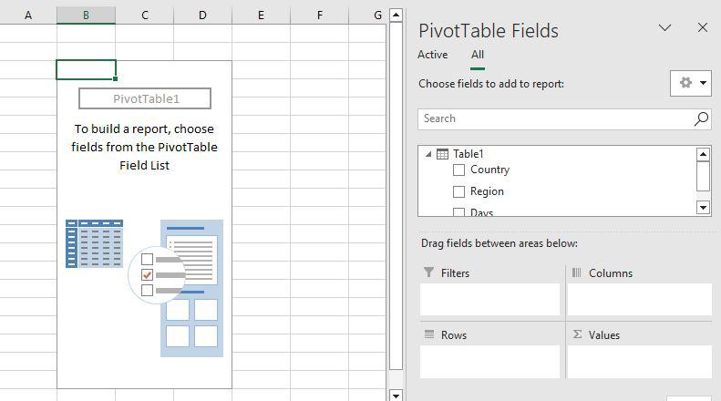
**Step 4: Add Fields to the Pivot Table
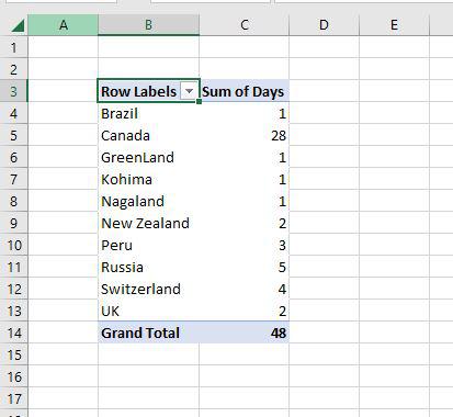
Drag the "Country" field to the Row area and the "Days" field to the Value area.
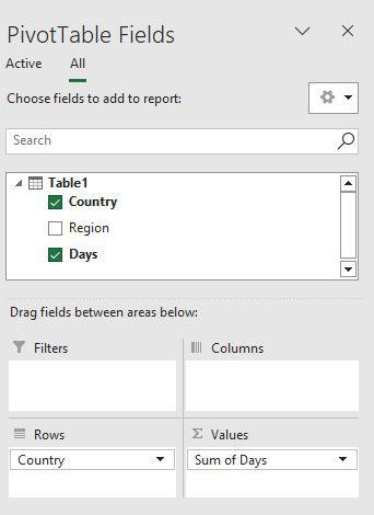
**Step 5: View the Complete Pivot Table
The pivot table will now display the data with "Country" and "Days" fields arranged accordingly.