Natural Language Processing (NLP) Pipeline (original) (raw)

Last Updated : 23 Jul, 2025

Natural Language Processing is referred to as NLP. It is a subset of artificial intelligence that enables machines to comprehend and analyze human languages. Text or audio can be used to represent human languages.

The natural language processing (NLP) pipeline refers to the sequence of processes involved in analyzing and understanding human language. The following is a typical NLP pipeline:

• Text & Speech processing
• Sentiment analysis
• Information Extraction
• Text Summarization
• Text generation
• Automatic Question Answering (chat-bot)
• Language Translation

The basic processes for all the above tasks are the same. Here we have discussed some of the most common approaches which are used during the processing of text data.

NLP Pipeline

In comparison to general machine learning pipelines, In NLP we need to perform some extra processing steps. The region is very simple that machines don't understand the text. Here our biggest problem is How to make the text understandable for machines. Some of the most common problems we face while performing NLP tasks are mentioned below.

1. Data Acquisition
2. Text Cleaning
3. Text Preprocessing
4. Feature Engineering
5. Model Building
6. Evaluation
7. Deployment

NLP Pipeline

1. Data Acquisition :

As we know, For building the machine learning model we need data related to our problem statements, Sometimes we have our data and Sometimes we have to find it. Text data is available on websites, in emails, in social media, in form of pdf, and many more. But the challenge is. Is it in a machine-readable format? if in the machine-readable format then will it be relevant to our problem? So, First thing we need to understand our problem or task then we should search for data. Here we will see some of the ways of collecting data if it is not available in our local machine or database.

• Public Dataset: We can search for publicly available data as per our problem statement.
• Web Scrapping: Web Scrapping is a technique to scrap data from a website. For this, we can use Beautiful Soup to scrape the text data from the web page.
• Image to Text: We can also scrap the data from the image files with the help of Optical character recognition (OCR). There is a library Tesseract that uses OCR to convert image to text data.
• pdf to Text: We have multiple Python packages to convert the data into text. With the PyPDF2 library, pdf data can be extracted in the .text file.
• Data augmentation: if our acquired data is not very sufficient for our problem statement then we can generate fake data from the existing data by Synonym replacement, Back Translation, Bigram flipping, or Adding some noise in data. This technique is known as Data augmentation.

2. Text Cleaning :

Sometimes our acquired data is not very clean. it may contain HTML tags, spelling mistakes, or special characters. So, let's see some techniques to clean our text data.

• Unicode Normalization: if text data may contain symbols, emojis, graphic characters, or special characters. Either we can remove these characters or we can convert this to machine-readable text. Python3 `

Unicode Nomalization

text = "GeeksForGeeks ????" print(text.encode('utf-8'))

text1 = 'गीक्स फॉर गीक्स ????' print(text1.encode('utf-8'))

`

Output :

b'GeeksForGeeks \xf0\x9f\x98\x80' b'\xe0\xa4\x97\xe0\xa5\x80\xe0\xa4\x95\xe0\xa5\x8d\xe0\xa4\xb8 \xe0\xa4\xab\xe0\xa5\x89\xe0\xa4\xb0 \xe0\xa4\x97\xe0\xa5\x80\xe0\xa4\x95\xe0\xa5\x8d\xe0\xa4\xb8 ????'

• Regex or Regular Expression: Regular Expression is the tool that is used for searching the string of specific patterns. Suppose our data contain phone number, email-Id, and URL. we can find such text using the regular expression. After that either we can keep or remove such text patterns as per requirements.
• Spelling corrections: When our data is extracted from social media. Spelling mistakes are very common in that case. To overcome this problem we can create a corpus or dictionary of the most common mistype words and replace these common mistakes with the correct word. Python3 `

import re text = """ #GFG Geeks Learning together url https://www.geeksforgeeks.org/, email acs@sdf.dv """ def clean_text(text): # remove HTML TAG html = re.compile('[<,#*?>]') text = html.sub(r'',text) # Remove urls: url = re.compile('https?://\S+|www.S+') text = url.sub(r'',text) # Remove email id: email = re.compile('[A-Za-z0-2]+@[\w]+.[\w]+') text = email.sub(r'',text) return text print(clean_text(text))

`

Output:

gfg GFG Geeks Learning together url
email

3. Text Preprocessing:

NLP software mainly works at the sentence level and it also expects words to be separated at the minimum level.

Our cleaned text data may contain a group of sentences. and each sentence is a group of words. So, first, we need to Tokenize our text data.

• Tokenization: Tokenization is the process of segmenting the text into a list of tokens. In the case of sentence tokenization, the token will be sentenced and in the case of word tokenization, it will be the word. It is a good idea to first complete sentence tokenization and then word tokenization, here output will be the list of lists. Tokenization is performed in each & every NLP pipeline.
• Lowercasing: This step is used to convert all the text to lowercase letters. This is useful in various NLP tasks such as text classification, information retrieval, and sentiment analysis.
• Stop word removal: Stop words are commonly occurring words in a language such as "the", "and", "a", etc. They are usually removed from the text during preprocessing because they do not carry much meaning and can cause noise in the data. This step is used in various NLP tasks such as text classification, information retrieval, and topic modeling.
• Stemming or lemmatization: Stemming and lemmatization are used to reduce words to their base form, which can help reduce the vocabulary size and simplify the text. Stemming involves stripping the suffixes from words to get their stem, whereas lemmatization involves reducing words to their base form based on their part of speech. This step is commonly used in various NLP tasks such as text classification, information retrieval, and topic modeling.
• Removing digit/punctuation: This step is used to remove digits and punctuation from the text. This is useful in various NLP tasks such as text classification, sentiment analysis, and topic modeling.
• POS tagging: POS tagging involves assigning a part of speech tag to each word in a text. This step is commonly used in various NLP tasks such as named entity recognition, sentiment analysis, and machine translation.
• Named Entity Recognition (NER): NER involves identifying and classifying named entities in text, such as people, organizations, and locations. This step is commonly used in various NLP tasks such as information extraction, machine translation, and question-answering. Python3 `

import nltk from nltk.tokenize import word_tokenize from nltk.corpus import stopwords from nltk.stem import SnowballStemmer, WordNetLemmatizer from nltk.tag import pos_tag from nltk.chunk import ne_chunk import string

sample text to be preprocessed

text = 'GeeksforGeeks is a very famous edutech company in the IT industry.'

tokenize the text

tokens = word_tokenize(text)

remove stop words

stop_words = set(stopwords.words('english')) filtered_tokens = [token for token in tokens if token.lower() not in stop_words]

perform stemming and lemmatization

stemmer = SnowballStemmer('english') lemmatizer = WordNetLemmatizer() stemmed_tokens = [stemmer.stem(token) for token in filtered_tokens] lemmatized_tokens = [lemmatizer.lemmatize(token) for token in filtered_tokens]

remove digits and punctuation

cleaned_tokens = [token for token in lemmatized_tokens if not token.isdigit() and not token in string.punctuation]

convert all tokens to lowercase

lowercase_tokens = [token.lower() for token in cleaned_tokens]

perform part-of-speech (POS) tagging

pos_tags = pos_tag(lowercase_tokens)

perform named entity recognition (NER)

named_entities = ne_chunk(pos_tags)

print the preprocessed text

print("Original text:", text) print("Preprocessed tokens:", lowercase_tokens) print("POS tags:", pos_tags) print("Named entities:", named_entities)

`

Output:

Original text: GeeksforGeeks is a very famous edutech company in the IT industry. Preprocessed tokens: ['geeksforgeeks', 'famous', 'edutech', 'company', 'industry'] POS tags: [('geeksforgeeks', 'NNS'), ('famous', 'JJ'), ('edutech', 'JJ'), ('company', 'NN'), ('industry', 'NN')] Named entities: (S geeksforgeeks/NNS famous/JJ edutech/JJ company/NN industry/NN)

Here, Stop word removal, Stemming and lemmatization, Removing digit/punctuation, and lowercasing are the most common steps used in most of the pipelines.

4 . Feature Engineering:

In Feature Engineering, our main agenda is to represent the text in the numeric vector in such a way that the ML algorithm can understand the text attribute. In NLP this process of feature engineering is known as Text Representation or Text Vectorization.

There are two most common approaches for Text Representation.

1. Classical or Traditional Approach:

In the traditional approach, we create a vocabulary of unique words assign a unique id (integer value) for each word. and then replace each word of a sentence with its unique id. Here each word of vocabulary is treated as a feature. So, when the vocabulary is large then the feature size will become very large. So, this makes it tough for the ML model.

One Hot Encoder:

One Hot Encoding represents each token as a binary vector. First mapped each token to integer values. and then each integer value is represented as a binary vector where all values are 0 except the index of the integer. index of the integer is marked by 1.

Python3 `

import nltk

nltk.download('punkt') # Download 'punkt'

from nltk if it's not downloaded

from nltk.tokenize import sent_tokenize Text = """Geeks For Geeks. Geeks Learning Together. Geeks For Geeks is famous for DSA. Learning DSA""" sentences = sent_tokenize(Text) sentences = [sent.lower().replace(".", "") for sent in sentences] print('Tokenized Sentences :', sentences)

Create the vocabulary

vocab = {} count = 0 for sent in sentences: for word in sent.split(): if word not in vocab: count = count + 1 vocab[word] = count print('vocabulary :', vocab)

One Hot Encoding

def OneHotEncoder(text): onehot_encoded = [] for word in text.split(): temp = [0]*len(vocab) if word in vocab: temp[vocab[word]-1] = 1 onehot_encoded.append(temp) return onehot_encoded

print('\n',sentences[0])

print('OneHotEncoded vector for sentence : "', sentences[0], '"is \n', OneHotEncoder(sentences[0]))

`

Output:

Tokenized Sentences : ['geeks for geeks', 'geeks learning together', 'geeks for geeks is famous for dsa', 'learning dsa'] vocabulary : {'geeks': 1, 'for': 2, 'learning': 3, 'together': 4, 'is': 5, 'famous': 6, 'dsa': 7} OneHotEncoded vector for sentence : " geeks for geeks "is
[[1, 0, 0, 0, 0, 0, 0], [0, 1, 0, 0, 0, 0, 0], [1, 0, 0, 0, 0, 0, 0]]

Bag of Word(Bow):

A bag of words only describes the occurrence of words within a document or not. It just keeps track of word counts and ignores the grammatical details and the word order.

Code block

Python3 `

import nltk #nltk.download('punkt') # Download 'punkt' from nltk if it's not downloaded from nltk.tokenize import sent_tokenize from sklearn.feature_extraction.text import CountVectorizer Text = """GeeksForGeeks. Geeks Learning Together. GeeksForGeeks is famous for DSA. Learning DSA"""

TOKENIZATION

sentences = sent_tokenize(Text) sentences = [sent.lower().replace(".","") for sent in sentences] print('Our Corpus:',sentences) #CountVectorizer : Convert a collection of text documents to a matrix of token counts. count_vect = CountVectorizer()

fit & transform will represent each sentences as BOW representation

BOW = count_vect.fit_transform(sentences)

Get the vocabulary

print("Our vocabulary: ", count_vect.vocabulary_) #see the BOW representation print(f"BoW representation for {sentences[0]} {BOW[0].toarray()}") print(f"BoW representation for {sentences[1]} {BOW[1].toarray()}") print(f"BoW representation for {sentences[2]} {BOW[2].toarray()}")

BOW representation for a new text

BOW_ = count_vect.transform(["learning dsa from geeksforgeeks"]) print("Bow representation for 'learning dsa from geeksforgeeks':", BOW_.toarray())

`

Output:

Our Corpus: ['geeksforgeeks', 'geeks learning together', 'geeksforgeeks is famous for dsa', 'learning dsa'] Our vocabulary: {'geeksforgeeks': 4, 'geeks': 3, 'learning': 6, 'together': 7, 'is': 5, 'famous': 1, 'for': 2, 'dsa': 0} BoW representation for geeksforgeeks [[0 0 0 0 1 0 0 0]] BoW representation for geeks learning together [[0 0 0 1 0 0 1 1]] BoW representation for geeksforgeeks is famous for dsa [[1 1 1 0 1 1 0 0]] Bow representation for 'learning dsa from geeksforgeeks': [[1 0 0 0 1 0 1 0]]

Bag of n-grams:

In Bag of Words, there is no consideration of the phrases or word order. Bag of n-gram tries to solve this problem by breaking text into chunks of n continuous words.

Python3 `

import nltk

nltk.download('punkt') # Download 'punkt'

from nltk if it's not downloaded

from nltk.tokenize import sent_tokenize from sklearn.feature_extraction.text import CountVectorizer

Text = """GeeksForGeeks. Geeks Learning Together. GeeksForGeeks is famous for DSA. Learning DSA"""

TOKENIZATION

sentences = sent_tokenize(Text) sentences = [sent.lower().replace(".", "") for sent in sentences] print('Our Corpus:', sentences)

Ngram vectorization example with count

vectorizer and uni, bi, trigrams

count_vect = CountVectorizer(ngram_range=(1, 3))

fit & transform will represent each sentences

as Bag of n-grams representation

BOW_nGram = count_vect.fit_transform(sentences)

Get the vocabulary

print("Our vocabulary:\n", count_vect.vocabulary_)

see the Bag of n-grams representation

print('Ngram representation for "{}" is {}' .format(sentences[0], BOW_nGram[0].toarray())) print('Ngram representation for "{}" is {}' .format(sentences[1], BOW_nGram[1].toarray())) print('Ngram representation for "{}" is {}'. format(sentences[2], BOW_nGram[2].toarray()))

Bag of n-grams representation for a new text

BOW_nGram_ = count_vect.transform(["learning dsa from geeksforgeeks together"]) print("Ngram representation for 'learning dsa from geeksforgeeks together' is", BOW_nGram_.toarray())

`

Output:

Our Corpus: ['geeksforgeeks', 'geeks learning together', 'geeksforgeeks is famous for dsa', 'learning dsa'] Our vocabulary: {'geeksforgeeks': 9, 'geeks': 6, 'learning': 15, 'together': 18, 'geeks learning': 7, 'learning together': 17, 'geeks learning together': 8, 'is': 12, 'famous': 1, 'for': 4, 'dsa': 0, 'geeksforgeeks is': 10, 'is famous': 13, 'famous for': 2, 'for dsa': 5, 'geeksforgeeks is famous': 11, 'is famous for': 14, 'famous for dsa': 3, 'learning dsa': 16} Ngram representation for "geeksforgeeks" is [[0 0 0 0 0 0 0 0 0 1 0 0 0 0 0 0 0 0 0]] Ngram representation for "geeks learning together" is [[0 0 0 0 0 0 1 1 1 0 0 0 0 0 0 1 0 1 1]] Ngram representation for "geeksforgeeks is famous for dsa" is [[1 1 1 1 1 1 0 0 0 1 1 1 1 1 1 0 0 0 0]] Ngram representation for 'learning dsa from geeksforgeeks together' is [[1 0 0 0 0 0 0 0 0 1 0 0 0 0 0 1 1 0 1]]

The output shows that the input text has been tokenized into sentences and processed to remove any periods and convert to lowercase. The vectorizer then computes the Bag of n-grams representation of each sentence, and the vocabulary used by the vectorizer is printed. Finally, the n-gram representation of a new text is computed and printed. The n-gram representations are in the form of a sparse matrix, where each row represents a sentence and each column represents an n-gram in the vocabulary. The values in the matrix indicate the frequency of the corresponding n-gram in the sentence.

TF-IDF (Term Frequency - Inverse Document Frequency):

In all the above techniques, Each word is treated equally. TF-IDF tries to quantify the importance of a given word relative to the other word in the corpus. it is mainly used in Information retrieval.

• Term Frequency (TF): TF measures how often a word occurs in the given document. it is the ratio of the number of occurrences of a term or word (t ) in a given document (d) to the total number of terms in a given document (d).

\text{TF}(t,d) = \frac{\text{(Number of occurrences of term t in document d)}} {\text{(Total number of terms in the document d)}}

• Inverse document frequency (IDF): IDF measures the importance of the word across the corpus. it down the weight of the terms, which commonly occur in the corpus, and up the weight of rare terms.

\text{IDF}(t)= \log_{e}\frac{\text{(Total number of documents in the corpus)}} {\text{(Number of documents with term t in corpus)}}

• TF-IDF score is the product of TF and IDF.

\text{TF-IDF Score} = TF\;\times \;IDF

Python3 `

import nltk

nltk.download('punkt') # Download 'punkt'

from nltk if it's not downloaded

from nltk.tokenize import sent_tokenize from sklearn.feature_extraction.text import TfidfVectorizer

Text = """GeeksForGeeks. Geeks Learning Together. GeeksForGeeks is famous for DSA. Learning DSA"""

TOKENIZATION

sentences = sent_tokenize(Text) sentences = [sent.lower().replace(".", "") for sent in sentences] print('Our Corpus:', sentences)

TF-IDF

tfidf = TfidfVectorizer() tfidf_matrix = tfidf.fit_transform(sentences)

All words in the vocabulary.

print("vocabulary", tfidf.get_feature_names())

IDF value for all words in the vocabulary

print("IDF for all words in the vocabulary :\n", tfidf.idf_)

TFIDF representation for all documents in our corpus

print('\nTFIDF representation for "{}" is \n{}' .format(sentences[0], tfidf_matrix[0].toarray())) print('TFIDF representation for "{}" is \n{}' .format(sentences[1], tfidf_matrix[1].toarray())) print('TFIDF representation for "{}" is \n{}' .format(sentences[2],tfidf_matrix[2].toarray()))

TFIDF representation for a new text

matrix = tfidf.transform(["learning dsa from geeksforgeeks"]) print("\nTFIDF representation for 'learning dsa from geeksforgeeks' is\n", matrix.toarray())

`

Output:

Our Corpus: ['geeksforgeeks', 'geeks learning together', 'geeksforgeeks is famous for dsa', 'learning dsa'] vocabulary ['dsa', 'famous', 'for', 'geeks', 'geeksforgeeks', 'is', 'learning', 'together'] IDF for all words in the vocabulary : [1.51082562 1.91629073 1.91629073 1.91629073 1.51082562 1.91629073 1.51082562 1.91629073] TFIDF representation for "geeksforgeeks" is [[0. 0. 0. 0. 1. 0. 0. 0.]] TFIDF representation for "geeks learning together" is [[0. 0. 0. 0.61761437 0. 0. 0.48693426 0.61761437]] TFIDF representation for "geeksforgeeks is famous for dsa" is [[0.38274272 0.48546061 0.48546061 0. 0.38274272 0.48546061 0. 0. ]] TFIDF representation for 'learning dsa from geeksforgeeks' is [[0.57735027 0. 0. 0. 0.57735027 0. 0.57735027 0. ]]

Neural Approach (Word embedding):

The above technique is not very good for complex tasks like Text Generation, Text summarization, etc. and they can't understand the contextual meaning of words. But in the neural approach or word embedding, we try to incorporate the contextual meaning of the words. Here each word is represented by real values as the vector of fixed dimensions.

For example :

airplane =[0.7, 0.9, 0.9, 0.01, 0.35] kite =[0.7, 0.9, 0.2, 0.01, 0.2]

Here each value in the vector represents the measurements of some features or quality of the word which is decided by the model after training on text data. This is not interpretable for humans but Just for representation purposes. We can understand this with the help of the below table.

| | airplane | kite | | | ---------- | ---- | ---- | | Sky | 0.7 | 0.7 | | Fly | 0.9 | 0.9 | | Transport | 0.9 | 0.2 | | Animal | 0.01 | 0.01 | | Eat | 0.35 | 0.2 |

Now, The problem is how can we get these word embedding vectors.

There are following ways to deal with this.

1. Train our own embedding layer:

There are two ways to train our own word embedding vector :

• CBOW (Continuous Bag of Words): In this case, we predict the center word from the given set of context words i.e previous and afterwords of the center word.

For example :

I am learning Natural Language Processing from GFG.

I am learning Natural _____?_____ Processing from GFG.

CBOW

• SkipGram: In this case, we predict the context word from the center word.

For example :

I am learning Natural Language Processing from GFG.

I am __?___ _____?_____ Language ___?___ ____?____ GFG.

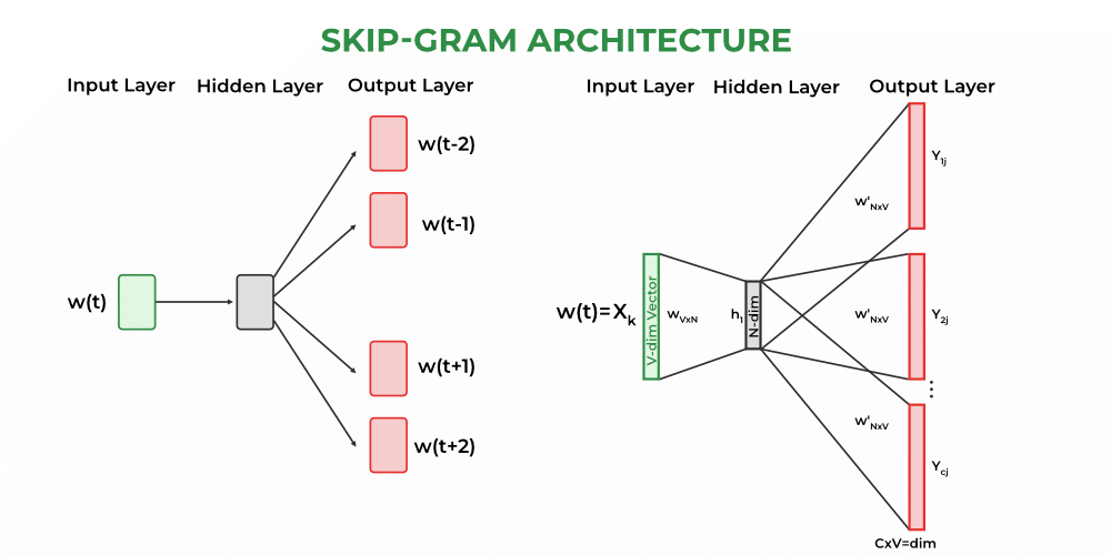
Skip-Gram

2. Pre-Trained Word Embeddings :

These models are trained on a very large corpus. We import from Gensim or Hugging Face and used it according to our purposes.

Some of the most popular pre-trained embeddings are as follows :

• Word2vec by Google Python3 `

import gensim.downloader as api

load the pre-trained Word2Vec model

model = api.load('word2vec-google-news-300')

define word pairs to compute similarity for

word_pairs = [('learn', 'learning'), ('india', 'indian'), ('fame', 'famous')]

compute similarity for each pair of words

for pair in word_pairs: similarity = model.similarity(pair[0], pair[1]) print(f"Similarity between '{pair[0]}' and '{pair[1]}' using Word2Vec: {similarity:.3f}")

`

Output:

Similarity between 'learn' and 'learning' using Word2Vec: 0.637 Similarity between 'india' and 'indian' using Word2Vec: 0.697 Similarity between 'fame' and 'famous' using Word2Vec: 0.326

• GloVe by Stanford Python3 `

import torch import torchtext.vocab as vocab

load the pre-trained GloVe model

glove = vocab.GloVe(name='840B', dim=300)

define word pairs to compute similarity for

word_pairs = [('learn', 'learning'), ('india', 'indian'), ('fame', 'famous')]

compute similarity for each pair of words

for pair in word_pairs: vec1, vec2 = glove[pair[0]], glove[pair[1]] similarity = torch.dot(vec1, vec2) / (torch.norm(vec1) * torch.norm(vec2)) print(f"Similarity between '{pair[0]}' and '{pair[1]}' using GloVe: {similarity:.3f}")

`

Output:

Similarity between 'learn' and 'learning' using GloVe: 0.768 Similarity between 'india' and 'indian' using GloVe: 0.764 Similarity between 'fame' and 'famous' using GloVe: 0.507

• fasttext by Facebook Python3 `

import gensim.downloader as api

load the pre-trained fastText model

fasttext_model = api.load("fasttext-wiki-news-subwords-300")

define word pairs to compute similarity for

word_pairs = [('learn', 'learning'), ('india', 'indian'), ('fame', 'famous')]

compute similarity for each pair of words

for pair in word_pairs: similarity = fasttext_model.similarity(pair[0], pair[1]) print(f"Similarity between '{pair[0]}' and '{pair[1]}' using Word2Vec: {similarity:.3f}")

`

Output:

Similarity between 'learn' and 'learning' using Word2Vec: 0.642 Similarity between 'india' and 'indian' using Word2Vec: 0.708 Similarity between 'fame' and 'famous' using Word2Vec: 0.519

5. Model Building:

Heuristic-Based Model

At the start of any project. When we have no very fewer data, then we can use a heuristic approach. The heuristic-based approach is also used for the data-gathering tasks for ML/DL model. Regular expressions are largely used in this type of model.

• Lexicon-Based-Sentiment- Analysis: Works by counting Positive and Negative words in sentences.
• Wordnet: It has a database of words with synonyms, hyponyms, and meronyms. It uses this database for solving rule-based NLP tasks.

Machine Learning Model:

• Naive Bayes: It is used for the classification task. It is a group of classification algorithms based on Bayes’ Theorem. It assumes that each feature has an equal and independent contribution to the outcomes. Naive Bayes is often used for document classification tasks, such as sentiment analysis or spam filtering.
• Support Vector Machine: This is also used for classification tasks. It is a popular supervised learning algorithm used for classification and regression analysis. It attempts to find the best hyperplane that separates the data points into different classes while maximizing the margin between the hyperplane and the closest data points. In the context of NLP, SVM is often used for text classification tasks, such as sentiment analysis or topic classification.
• Hidden Markov Model: HMM is a statistical model used to represent a sequence of observations that are generated by a sequence of hidden states. In the context of NLP, HMM is often used for speech recognition, part-of-speech tagging, and named entity recognition. HMM assumes that the state transitions are dependent only on the current state and the observation is dependent only on the current state.
• Conditional Random Fields: CRF is a type of probabilistic graphical model used for modeling sequential data where the output is a sequence of labels. It is similar to HMM, but unlike HMM, CRF can take into account more complex dependencies between the output labels. In the context of NLP, CRF is often used for named entity recognition, part-of-speech tagging, and information extraction. CRF can handle more complex input features, making it more powerful than HMM.

Deep Learning Model :

Recurrent neural networks

Recurrent neural networks are a particular class of artificial neural networks that are created with the goal of processing sequential or time series data. It is primarily used for natural language processing activities including language translation, speech recognition, sentiment analysis, natural language production, summary writing, etc. Unlike feedforward neural networks, RNNs include a loop or cycle built into their architecture that acts as a "memory" to hold onto information over time. This distinguishes them from feedforward neural networks. This enables the RNN to process data from sources like natural languages, where context is crucial.

The basic concept of RNNs is that they analyze input sequences one element at a time while maintaining track in a hidden state that contains a summary of the sequence’s previous elements. The hidden state is updated at each time step based on the current input and the previous hidden state. This allows RNNs to capture the temporal dependencies between elements of the sequence and use that information to make predictions.

Recurrent neural networks

Working: The fundamental component of an RNN is the recurrent neuron, which receives as inputs the current input vector and the previous hidden state and generates a new hidden state as output. And this output hidden state is then used as the input for the next recurrent neuron in the sequence. An RNN can be expressed mathematically as a sequence of equations that update the hidden state at each time step:

St= f(USt-1+Wxt+b)

Where,

• St = Current state at time t
• xt = Input vector at time t
• St-1 = Previous state at time t-1
• U = Weight matrix of recurrent neuron for the previous state
• W = Weight matrix of input neuron
• b = Bias added to the input vector and previous hidden state
• f = Activation functions

And the output of the RNN at each time step will be:

yt = g(VSt+c)

Where,

• yt = Output at time t
• V = Weight matrix for the current state in the output layer
• C = Bias for the output transformations.
• g = activation function

Here, W, U, V, b, and c are the learnable parameters and it is optimized during the backpropagation.

Models have to process a large number of tokens. When it is processing a distant token from the first token, The significance of the first token starts decreasing, So, it fails to relate with starting token to the distant token. This can be avoided with explicit state management by using gates.

There are two architectures that try to solve this problem.

• Long short-term memory (LSTM)
• Gated relay unit (GRU)

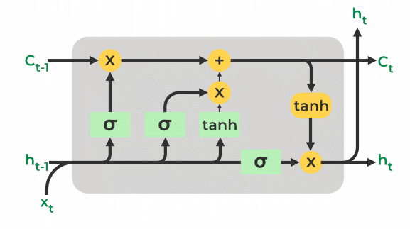
Long Short-Term Memory (LSTM):

Long Short-Term Memory Networks are an advanced form of RNN model, and it handles the vanishing gradient problem of RNN. It only remembers the part of the context which has a meaningful role in predicting the output value. LSTMs function by selectively passing or retaining information from one-time step to the next using the combination of memory cells and gating mechanisms.

Long Short-Term Memory (LSTM)

The LSTM cell is made up of a number of parts, such as:

• Cell state (C): The LSTM's memory component is where the information from the preceding phase is stored at this time. Gates that regulate the flow of data into and out of the LSTM cell are used to pass it through.
• Hidden state (h): This is the LSTM cell's output, which is a modified representation of the cell state. It may be applied to predictions or transferred to a subsequent LSTM cell in the sequence.
• Forget gate (f): The forget gate removes the data that is no longer relevant in the cell state. The gate receives two inputs, xt (input at the current time) and ht-1 (previous hidden state), which are multiplied with weight matrices, and bias is added. The result is passed via an activation function, which gives a binary output i.e. True or False.
• Input Gate(i): The input gate determines what parts of the input should be added to the cell state by applying a sigmoid activation function to the current input and the previous concealed state as inputs. The new values that are added to the cell state are created by multiplying the output of the input gate (again, a fraction between 0 and 1) by the output of the tanh block. The current cell state is created by adding this gated vector to the previous cell state.
• Output Gate(o): The output gate takes the crucial data and outputs it from the state of the current cell. First, a vector is created in the cell using the tanh function. The data is then filtered by the values to be remembered using the inputs ht-1 and xt, and the information is then controlled using the sigmoid function. The vector's values and the controlled values are finally multiplied and supplied as input and output to the following cell, respectively.
  The two-state vector for LSTM represents the current state.

GRU (Gated Recurrent Unit):

Gated Recurrent Unit (GRU) is also the advanced form of RNN. which solves the vanishing gradient problem. Like LSTMs, GRUs also have gating mechanisms that allow them to selectively update or forget information from the previous time steps. However, GRUs have fewer parameters than LSTMs, which makes them faster to train and less prone to overfitting. The two gates in GRUs are the reset gate and the update gate, which control the flow of information in the network.

GRU (Gated Recurrent Unit):

• Update Gate: this controls the amount of information passed through the next state.
• Rest Gate: It decides whether the previous cell state is important or not.

6. Evaluation :

Evaluation matric depends on the type of NLP task or problem. Here I am listing some of the popular methods for evaluation according to the NLP tasks.

• Classification: Accuracy, Precision, Recall, F1-score, AUC
• Sequence Labelling: Fl-Score
• Information Retrieval : Mean Reciprocal rank(MRR), Mean Average Precision (MAP),
• Text summarization: ROUGE
• Regression [Stock Market Price predictions, Temperature Predictions]: Root Mean Square Error, Mean Absolute Percentage Error
• Text Generation: BLEU (Bi-lingual Evaluation Understanding), Perplexity
• Machine Translation: BLEU (Bi-lingual Evaluation Understanding), METEOR

7. Deployment

Making a trained NLP model usable in a production setting is known as deployment. The precise deployment process can vary based on the platform and use case, however, the following are some typical processes that may be involved:

1. Export the trained model: The trained model must first be exported from the training environment in order to be loaded and used in a production environment. This may entail preserving the model's architecture, parameters, and any additional pertinent artifacts, like vocabulary or embeddings.
2. Prepare the input pipeline: It is required to set up the input pipeline such that the input data is preprocessed in the same manner as it was during training before the model can be used to produce predictions. Depending on the specific NLP task, this may require tokenization, normalization, or other preparatory procedures.
3. Set up the inference service: Setting up an inference service that can provide predictions using the trained model comes next after the input pipeline has been installed. To accomplish this, it may be necessary to build up a web server or other API endpoint that can accept requests containing input data, preprocess it using the input pipeline, and then give it to the model for prediction.
4. Monitor performance and scale: Following deployment, it is crucial to keep an eye on the model's performance and adjust scaling as necessary to manage variations in traffic and demand. Setting up performance metrics to monitor the model's effectiveness and modifying the infrastructure as necessary to ensure optimal performance may be required.
5. Continuous improvement: Finally, it's important to keep an eye on and develop the deployed model over time. This could entail getting user feedback, retraining the model with fresh data, or adjusting the model's parameters or architecture to boost performance.