Pandas Step by Step Guide (original) (raw)
Last Updated : 9 Jun, 2026
Pandas is a popular open-source Python library used for data manipulation and analysis. It provides powerful tools for working with structured data and integrates seamlessly with libraries such as NumPy and Matplotlib. Pandas operates around two core data structures:
- **Series (1D): Used to handle single columns of data efficiently.
- **DataFrame (2D): Used for structured, tabular data similar to spreadsheets or SQL tables.
1. Installing and Importing Pandas
To install Pandas, run the following command in your terminal or command prompt:
pip install pandas
After installation, import Pandas into your Python script or notebook using the standard alias pd.
Python `
import pandas as pd
`
**2. Creating DataFrames
A DataFrame is a two-dimensional table with labeled rows and columns, similar to a spreadsheet or SQL table. Each column can store different data types, such as numbers, text, or dates. DataFrames can be created from lists, dictionaries, or other data sources.
**Example: Creating a DataFrame using a Dictionary
In this example, a dictionary is converted into a DataFrame using the pd.DataFrame() function.
Python `
import pandas as pd
data = { 'Name': ["Player_A", "Player_B", "Player_C"], 'Age': [25, 30, 35]}
df = pd.DataFrame(data)
print(df)
`
**Output:
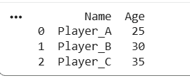
DataFrame
3. Creating Series
A Series is a one-dimensional labeled array that can store any data type, such as integers, strings, or floats. Each value is associated with an index, which can be default (0, 1, 2, ...) or custom labels. Series can be created from lists, NumPy arrays, dictionaries, or scalar values.
**Example: Creating a Series using a List
Python `
import pandas as pd age_series = pd.Series([25, 30, 35], index=["Player_A", "Player_B", "Player_C"]) print(age_series)
`
**Output:
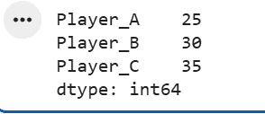
Series
4. Reading CSV and JSON Files
CSV (Comma-Separated Values) files are commonly used to store tabular data. Pandas provides the read_csv() function to load a CSV file into a DataFrame. By default, Pandas displays only a preview of large datasets. To display all rows, you can use to_string() or adjust the pd.options.display.max_rows setting.
Python `
import pandas as pd df = pd.read_csv("people.csv") print(df)
`
**Output:

Pandas Read CSV
Pandas supports multiple file formats such as CSV and JSON (JavaScript Object Notation). You can load a JSON file into a DataFrame using the read_json() function.
Python `
import pandas as pd
df = pd.read_json('data.json')
`
**5. Understanding and Analyzing the Data Frame
After creating or loading a DataFrame, inspecting and summarizing the data is an important step in understanding dataset. Pandas provides various functions to help you view and analyze the data.
- **head():View the first n rows of the DataFrame (default is 5 rows).
- **tail(): View the last n rows of the DataFrame (default is 5 rows).
- **info():Shows a summary of the DataFrame, including column names, data types, and non-null values.
- **describe():Provides summary statistics such as count, mean, and standard deviation for numerical columns. Use describe(include="all") to include non-numeric data.
Let's see an example demonstrating the use of .head(), .tail(), .info() and .describe() methods:
Python `
import pandas as pd
data = {'Name': ['Alice', 'Bob', 'Charlie', 'David', 'Eva'], 'Age': [24, 27, 22, 32, 29], 'City': ['New York', 'Los Angeles', 'Chicago', 'Houston', 'Phoenix']} df = pd.DataFrame(data)
print("First 3 rows using head():") print(df.head(3))
print("\nLast 2 rows using tail():") print(df.tail(2))
print("\nDataFrame summary using info():") df.info()
`
**Output:
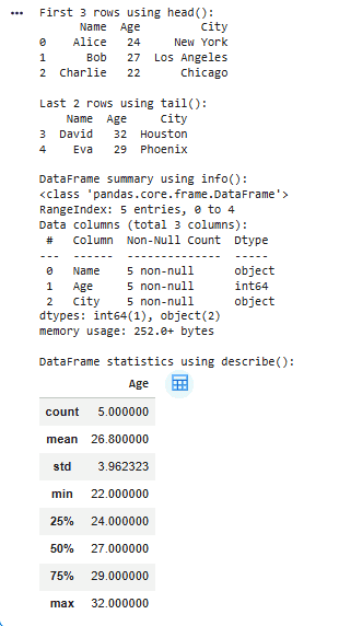
Understanding Data in Pandas
Pandas provides versatile tools to inspect and understand data quickly. These functions help in summarizing datasets and exploring key attributes efficiently.
- View basic statistical details
- Get information about the DataFrame (data types, non-null counts, etc.)
- Check for missing data
- Inspect the DataFrame shape (rows and columns)
- Checking rows with minimum and maximum values
6. Indexing in Pandas
Indexing in Pandas refers to accessing and selecting data from a DataFrame or Series. There are multiple ways to do this, including selecting columns, slicing data, and filtering using conditions.
**Example : Basic Indexing (Selecting a single column) with use of [ ] operator.
Python `
import pandas as pd
data = {'Name': ['Alice', 'Bob', 'Charlie'],'Age': [25, 30, 35]} df = pd.DataFrame(data)
age_column = df['Age'] print(age_column)
`
**Output:
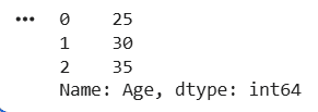
Indexing
We can also select multiple columns by passing a list of column names, such as ['Name', 'Age'], which returns a new DataFrame. Pandas provides two main methods for selecting rows:
- ****.loc[]** : Label-based indexing using row/column names or index labels.
- ****.iloc[]** : Position-based indexing using integer positions (0, 1, 2, ...). Python `
import pandas as pd
data = {'Name': ['Alice', 'Bob', 'Charlie'], 'Age': [25, 30, 35]} df = pd.DataFrame(data)
row_by_label = df.loc[1]
row_by_position = df.iloc[1]
print("Row by label:\n", row_by_label) print("\nRow by position:\n", row_by_position)
`
**Output:
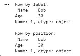
Indexing
For more advanced selection techniques, you can explore topics like selecting multiple columns, slicing, and Boolean indexing.
7. Selecting and Filtering Data Based on Conditions
Filtering data means selecting only those rows or columns that meet specific conditions instead of working with the entire dataset. This helps in extracting relevant data for analysis using logical conditions.
In the example below, we filter rows where the Age column is greater than 28, returning only matching records.
Python `
import pandas as pd
data = {'Name': ['Alice', 'Bob', 'Charlie'],'Age': [25, 30, 35]} df = pd.DataFrame(data) filtered_df = df[df['Age'] > 28]
print(filtered_df)
`
You can also refer to following resources for advanced techniques and more conditions in filtering and selection:
8. Dealing with Rows and Columns in Pandas DataFrame
It involves various data manipulation techniques in Pandas, such as adding and deleting columns, truncating data, iterating over DataFrames and sorting data. For more detailed explanations of each concept and step, you can refer to Dealing with Rows and Columns in Pandas DataFrame.
**1. Adding a New Column to DataFrame: We can easily add new columns by assigning values to them by direct assignment.
Python `
import pandas as pd
df = pd.DataFrame({'Name': ['Alice', 'Bob', 'Charlie'], 'Age': [25, 30, 35]})
df['Salary'] = [50000, 60000, 70000] print(df)
`
**Output:
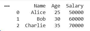
Adding a new column
There are multiple methods, for that refer to: Adding new column to existing dataFrame in pandas. If you want to add columns from one dataFrame to another, refer to Adding Columns from Another DataFrame.
**2. Renaming Columns in a DataFrame: We can use the rename() method for selective renaming of specific columns or directly modify the columns attribute when renaming all columns at once.
Python `
import pandas as pd
df = pd.DataFrame({'A': [1, 2, 3], 'B': [4, 5, 6], 'C': [7, 8, 9]})
df.rename(columns={'A': 'X', 'B': 'Y', 'C': 'Z'}, inplace=True) print(df)
`
**Output:
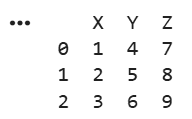
Renamed Columns
We can also Rename column by index in Pandas
**3. Reindexing Data with Pandas: Reindexing in Pandas is used to change the row or column labels of a DataFrame or Series. It helps align data with new labels, handle missing values, and restructure datasets. The reindex() method updates indices or column names as needed.
**Note: If the new index includes labels not present in the original DataFrame, the corresponding values will be set to NaN by default.
Python `
import pandas as pd
data = {'A': [10, 20, 30], 'B': [40, 50, 60]} df = pd.DataFrame(data)
new_index = [0, 1, 2, 3] df_reindexed = df.reindex(new_index) print("Reindexed Rows:\n", df_reindexed)
`
**Output:
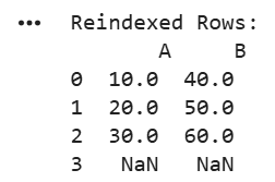
Reindexed Rows
What if you want to reset the index? for that refer to: Convert Index to Column in Pandas Dataframe
9. Handling Missing Data in Pandas
Working with missing data is one of the most common tasks in data manipulation. Pandas provides several functions to identify, fill, and remove missing values efficiently. This helps ensure data quality before performing analysis.
**1. Identifying Missing Data With Pandas using **isnull() and notnull():
isnull():True where values are missing (NaN) and False where values are present.notnull():
**Example:
Python `
import pandas as pd import numpy as np df = pd.DataFrame({'Col1': [1, 2, np.nan],'Col2': [3, np.nan, np.nan]})
print(df.isnull())
`
**Output:
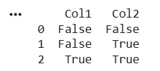
Checking Missing Values
When working with real world datasets, missing values are common. Broadly, we have two main ways to deal with missing data:
- Impute (Fill) the missing values
- Remove (Delete) the missing values
**2. Filling Missing Data: Missing values can be replaced using the fillna() method.
**For example: Replacing all missing values with 0. This method modifies the dataset directly when inplace=True is used.
Python `
import pandas as pd import numpy as np
df = pd.DataFrame({'Col1': [1, 2, np.nan],'Col2': [3, np.nan, np.nan]}) df.fillna(0,inplace=True)
print(df)
`
**Output:
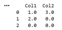
Filled Missing Values with 0
We can also fill missing values with below techniques:
**3. Dropping Missing Data With Pandas: We can remove missing values using the dropna() method. Depending on the requirement, Pandas allows different ways to drop data.
Common approaches include:
- Removing columns that contain missing values using df.dropna(axis=1)
- Dropping rows where certain columns have missing values using df.dropna(subset=['Column1', 'Column2'])
To explore more variations of dropping data, you can refer to topics like Dropping Rows from a Pandas DataFrame with Missing Values and Dropping One or Multiple Columns.
For example:
Python `
import pandas as pd
data = {'Name': ['Alice', 'Bob', None], 'Age': [25, None, 35]} df = pd.DataFrame(data) df_dropped = df.dropna()
print(df_dropped)
`
**Output:

Missing Data Dropped
10. Aggregation and Grouping With Pandas
Aggregation and grouping in Pandas are used to analyze and summarize data. Grouping divides data into categories, while aggregation performs operations like sum, mean, or count to extract insights.
The groupby() function is commonly used for grouping data, followed by aggregation functions like sum(), mean(), size(), or custom operations.
**Example:
- **groupby('Category'): Groups data by the 'Category' column.
- ****.sum(), .mean(), and .size():** Perform aggregation on the grouped data. Python `
import pandas as pd
data = {'Category': ['A', 'B', 'A', 'B'], 'Value': [10, 20, 30, 40]} df = pd.DataFrame(data)
grouped_sum = df.groupby('Category').sum() print("Sum:\n", grouped_sum)
grouped_mean = df.groupby('Category')['Value'].mean() print("\nMean:\n", grouped_mean)
grouped_agg = df.groupby('Category').agg(['sum', 'mean']) print("\nAggregated:\n", grouped_agg)
`
**Output:
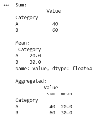
Grouping in Pandas
- For more detailed information and practical examples, refer Grouping and Aggregating with Pandas
- For more advanced operations, you can use
.agg()to apply custom aggregation functions.- Grouping Rows in pandas
11. Merging and Concatenating Data in Pandas
This section explains how to combine multiple DataFrames or Series into a single DataFrame. These operations are commonly used to integrate datasets and organize data for analysis.
**1. Merging DataFrames: Combines data based on common column or index using functions like merge or join. There are mainly 4 types of joins:
- **Inner Join: Keeps rows that match in both DataFrames.
- **Left Join: Keeps all rows from the left DataFrame and match data from the right.
- **Right Join and Outer Join: Keep similar but differ in data retention rules.
**Example:
Python `
import pandas as pd
data1 = { 'Name': ['Alice', 'Charlie', 'Edward', 'Grace'], 'Years_Experience': [2, 3, 4, 6] } df1 = pd.DataFrame(data1)
data2 = { 'Name': ['Alice', 'Charlie', 'Frank', 'Grace'], 'Role': ['Manager', 'Analyst', 'Developer', 'HR'] } df3 = pd.DataFrame(data2)
df_merged_inner = pd.merge(df1, df3, on='Name', how='inner')
df_merged_outer = pd.merge(df1, df3, on='Name', how='outer')
print("\nInner Merge (Intersection of Names):\n", df_merged_inner) print("\nOuter Merge (Union of Names):\n", df_merged_outer)
`
**Output:
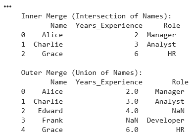
Merging in Pandas
**2. Concatenating Data: Concatenation is used to stack DataFrames either vertically (row-wise) or horizontally (column-wise) using pd.concat(). Let's create two dataFrames and concatenate it with the original one:
**Example:
- By default, pd.concat() concatenates DataFrames row-wise (axis=0), stacking them vertically.
- ignore_index=True resets the index to create a continuous sequence instead of keeping original indices. Python `
import pandas as pd
df = pd.DataFrame({ 'Name': ['Alice', 'Charlie', 'Edward', 'Grace'], 'Years_Experience': [2, 3, 4, 6], 'Role': ['Manager', 'Analyst', 'Developer', 'HR'] })
new_df = pd.DataFrame({ 'Name': ['John', 'Lily'], 'Years_Experience': [5, 3], 'Role': ['Designer', 'Developer'] })
concatenated_df = pd.concat([df, new_df], ignore_index=True)
print("Concatenated DataFrame:\n") print(concatenated_df)
`
**Output:
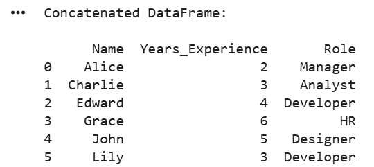
Concatenated Dataframe
- Learn Concatenate Two or More Pandas DataFrames with all operations and multiple examples. For more, Go Through below articles:
- Concatenate values in different columns to one column
- Merge two dataFrames on certain columns
- Merge multiple CSV Files into single dataframe
12. Reshaping Data in Pandas
Reshaping data means changing the structure of rows and columns to better organize or analyze data. Common operations include pivoting, melting, stacking, and unstacking.
**1. Pivot Tables in Pandas: Pivot tables reshape data based on column values and are useful for creating aggregated views using the pivot_table() method.
Python `
import pandas as pd
data = {'Date': ['2024-10-01', '2024-10-01', '2024-10-02', '2024-10-02'],'Category': ['A', 'B', 'A', 'B'],'Values': [10, 20, 15, 25]} df = pd.DataFrame(data)
pivot_table = df.pivot_table(values='Values', index='Date', columns='Category', aggfunc='sum') print(pivot_table)
`
**Output:
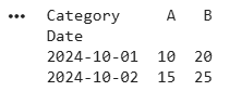
Pivoting in Pandas
**2. Melting : Multiple columns are combined into a single key value pair.
When you melt data:
- The column names become the keys.
- The values in the columns become the values.
**Note: To melt data, you must specify columns that act as "identifiers" (id_vars) and others that need to be melted (value_vars).
Python `
import pandas as pd
data = { 'Date': ['2024-10-01', '2024-10-01', '2024-10-02', '2024-10-02'], 'Category_A': [10, None, 15, None], 'Category_B': [None, 20, None, 25] }
df = pd.DataFrame(data)
melt_df = df.melt(id_vars='Date', var_name='Category', value_name='Value')
print(melt_df)
`
**Output:
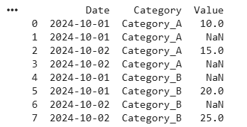
Melting in Pandas
**3. Stacking and Unstacking With Pandas: Reshapes data by changing rows and columns, especially useful with MultiIndex DataFrames. These methods help reorganize the structure of data for better analysis.
- **Stacking: Converts columns into rows, making the DataFrame taller.
- **Unstacking: Converts rows into columns, making the DataFrame wider.
**Example: When columns are stacked into rows using stack(), the DataFrame structure changes. The data now has a MultiIndex in the rows:
- First level Product (e.g., Product_A, Product_B)
- Second level Category (e.g., Sales, Expenses)
- The quarter values (Q1, Q2) remain as columns, while the higher level column labels move into the row index. Python `
import pandas as pd data = { ('Sales', 'Q1'): [100, 150], ('Sales', 'Q2'): [200, 250], ('Expenses', 'Q1'): [50, 70], ('Expenses', 'Q2'): [80, 90] }
index = ['Product_A', 'Product_B'] df = pd.DataFrame(data, index=index) print(df)
stacked_df = df.stack() print(stacked_df)
unstacked_df = stacked_df.unstack() print(unstacked_df)
`
**Output:
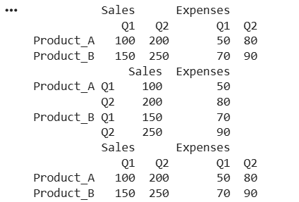
Stacking and Unstacking in Pandas
Let’s compare and understand in depth with more examples the stack(), unstack(), and melt() methods. We can also use the transpose() method to swap rows and columns when needed.
13. Handling Large Datasets With Pandas
When working with large datasets or heavy computations, performance optimization becomes important for faster processing and better memory usage. Pandas provides several techniques to improve efficiency.
- **Working with Chunks of Data****:** For datasets that don’t fit into memory, the chunksize parameter in pd.read_csv() be used to load data in parts. This allows processing data in smaller, manageable chunks instead of loading the entire dataset at once.
- **Optimizing Memory Usage by Changing Data Types****:** By default, Pandas may use larger data types (e.g.,
int64) even when not needed. Using .astype() to convert columns to smaller or more appropriate types helps reduce memory usage, especially in large datasets.
**Related Articles: