Classification in R Programming (original) (raw)

Last Updated : 30 Apr, 2026

Classification is a supervised machine learning technique used to assign data points into predefined categories based on their features. In R programming, classification models help build predictive systems that can automatically categorize new and unseen data. These models are widely used for tasks such as sentiment analysis, medical diagnosis, spam detection and recommendation systems.

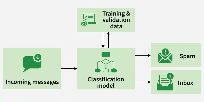
how Classification works

Classification Algorithms in R

R provides a wide range of powerful algorithms for solving classification problems. These algorithms help build predictive models that can accurately assign data into predefined categories based on patterns learned from training data.

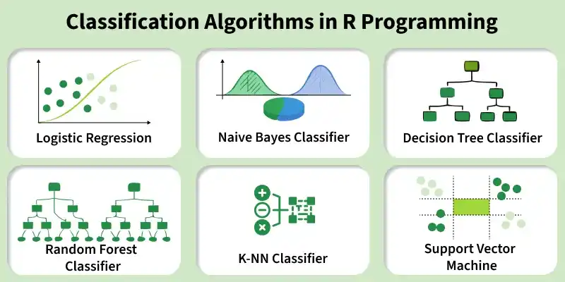
Classification Algorithms

1. Logistic Regression

Logistic Regression is a classification algorithm used to predict binary outcomes, such as Yes/No or 0/1. It estimates the probability that a data point belongs to a particular class based on its features and is widely applied in fields like healthcare, marketing, fraud detection and spam filtering.

Here we implements a logistic regression model in R to classify iris flowers as Setosa or Non-Setosa.

• Loads the iris dataset and converts the target variable Species into a binary factor.
• Fits a logistic regression model using Petal.Length and Petal.Width as predictors.
• Computes predicted probabilities, converts them into class labels using a 0.5 threshold and stores them as a factor.
• Uses ggplot2 to plot Petal.Length vs Petal.Width, coloring points by predicted class and shaping them by actual species. R `

library(ggplot2) data(iris) iris$Species <- factor(ifelse(iris$Species == "setosa", "Setosa", "Non-Setosa"), levels = c("Non-Setosa", "Setosa")) log_model <- glm(Species ~ Petal.Length + Petal.Width, data = iris, family = binomial)

iris$Predicted <- factor(ifelse(predict(log_model, type = "response") > 0.5, "Setosa", "Non-Setosa"), levels = c("Non-Setosa", "Setosa"))

ggplot(iris, aes(x = Petal.Length, y = Petal.Width, color = Predicted, shape = Species)) + geom_point(size = 3) + labs(title = "Logistic Regression Predictions") + theme_minimal()

`

**Output:

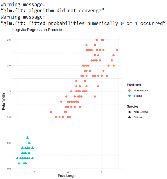
Output

2. Naive Bayes Classifier

Naive Bayes is a classification algorithm that predicts the category of a data point based on probabilities. It uses Bayes’ theorem to estimate how likely a data point belongs to each class, assuming that all features (predictors) are independent of each other. This makes the model fast to train and effective, especially for large datasets or text-based applications like spam detection.

Here we implements a Naive Bayes classifier in R to predict iris species and make predictions on the test set.

• Loads the necessary packages and the iris dataset, then splits it into training and testing sets.
• Scales the numeric features to normalize the data.
• Trains a Naive Bayes classifier on the training data using all features to predict Species.
• Uses the trained model to predict the species for the test set and stores the results in y_pred. R `

install.packages("e1071") install.packages("caTools") install.packages("caret")

library(e1071) library(caTools) library(caret) data(iris) set.seed(123) split <- sample.split(iris, SplitRatio = 0.7) train_cl <- subset(iris, split == TRUE) test_cl <- subset(iris, split == FALSE) train_scale <- scale(train_cl[, 1:4]) test_scale <- scale(test_cl[, 1:4]) classifier_cl <- naiveBayes(Species ~ ., data = train_cl) classifier_cl y_pred <- predict(classifier_cl, newdata = test_cl)

`

**Output:

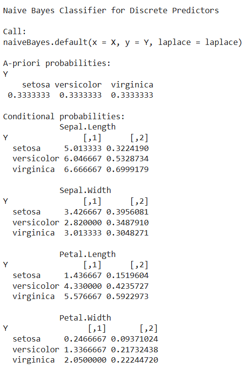
Output

3. Decision Tree Classifier

A Decision Tree Classifier is a supervised machine learning algorithm that predicts the class of a data point by splitting the dataset based on feature values into a tree-like structure. It is easy to interpret and widely used for classification tasks.

• Splits the dataset step by step based on feature values to create branches.
• Internal nodes represent features and decision points, while leaf nodes represent the predicted class.
• Helps make decisions or predictions in an easy to visualize tree format, useful for tasks like spam detection or medical diagnosis.

Here we implements a Decision Tree Classifier in R

• Loads the party package and the built-in iris dataset, then selects the first 100 rows for simplicity.
• Trains a Decision Tree using ctree() to predict Species based on Petal.Length and Petal.Width. R `

install.packages("party") library(party) data(iris) input.data <- iris[1:100, ] output.tree <- ctree(Species ~ Petal.Length + Petal.Width, data = input.data) plot(output.tree) plot(output.tree, type = "simple", horizontal = TRUE)

`

**Output:

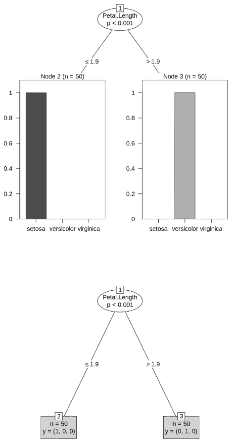
Decision Tree

This plots of Decision Tree showing how Petal.Length and Petal.Width are used to classify the iris species in the selected dataset.

4. Random Forest Classifier

Random Forest is an ensemble learning algorithm that builds multiple decision trees and combines their predictions to improve accuracy and reduce overfitting. For classification, it uses majority voting and for regression, it averages predictions. It is widely used in healthcare, finance and marketing for robust and reliable predictions.

• Builds multiple decision trees from random subsets of the data and features to create a “forest” of trees.
• Each tree makes a prediction and the class with the most votes becomes the final prediction for classification tasks.
• Reduces overfitting compared to a single decision tree, improving generalization to unseen data.
• Can handle large datasets with high dimensionality and works well with both numerical and categorical features.

Here we implements a Random Forest Classifier in R to predict a target variable and evaluate its performance.

• Splits the dataset into training and testing sets and converts the target variable to a factor for classification.
• Trains a Random Forest model using the caret package with the ranger method.
• Makes predictions on the test set, evaluates performance using a confusion matrix and displays feature importance. R `

install.packages("caret") install.packages("ranger") library(caret) library(ranger)

data(mtcars) mtcars$am <- factor(mtcars$am)

set.seed(123) train_index <- createDataPartition(mtcars$am, p = 0.7, list = FALSE) training_set <- mtcars[train_index, ] test_set <- mtcars[-train_index, ]

model_rf <- train(am ~ ., data = training_set, method = "ranger", importance = "impurity") predict_rf <- predict(model_rf, test_set)

cm_rf <- confusionMatrix(predict_rf, test_set$am) print(cm_rf) print(varImp(model_rf))

`

**Output:

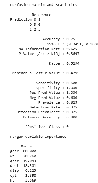
Output

5. K-NN Classifier

The K-Nearest Neighbors (K-NN) classifier is a non-parametric algorithm used for classification and regression. It predicts the class of a data point based on the majority class among its k closest neighbors in the feature space. K-NN is simple, intuitive and widely used in pattern recognition, economics, genetics and image recognition.

• Predicts the class of a data point by finding the k nearest points in the training dataset.
• Does not make assumptions about the underlying data distribution, making it non-parametric.
• Works well for datasets where similar points tend to belong to the same class.

Here we implements a K-NN classifier in R on the iris dataset and visualizes the predicted classes.

• Splits the iris dataset into training and testing sets using createDataPartition.
• Trains a K-NN model with k = 5 neighbors and predicts the species for the test set.
• Evaluates model performance with a confusion matrix and visualizes test points colored by predicted class using ggplot2. R `

install.packages("class") install.packages("caret") install.packages("ggplot2")

library(class) library(caret) library(ggplot2)

data(iris)

features <- iris[, c("Petal.Length", "Petal.Width")] labels <- iris$Species

set.seed(123) train_index <- createDataPartition(labels, p = 0.7, list = FALSE) train_features <- features[train_index, ] test_features <- features[-train_index, ] train_labels <- labels[train_index] test_labels <- labels[-train_index]

knn_pred <- knn(train_features, test_features, train_labels, k = 5)

print(confusionMatrix(knn_pred, test_labels))

test_data <- cbind(test_features, Predicted = knn_pred) ggplot(test_data, aes(x = Petal.Length, y = Petal.Width, color = Predicted)) + geom_point(size = 3) + labs(title = "K-NN Predictions on Iris Test Data") + theme_minimal()

`

**Output:

6. Support Vector Machine (SVM) Classifier

Support Vector Machines (SVMs) are supervised learning algorithms that classify data by finding the optimal hyperplane separating classes, maximizing the margin between support vectors. They are widely used in text classification, bioinformatics and image recognition for their accuracy and reliability on small to medium datasets.

• Finds the hyperplane that best separates classes by maximizing the margin between them.
• Uses support vectors (closest points to the hyperplane) to define the decision boundary.
• Can be extended for multiclass classification and can use kernels (linear, polynomial, RBF) to handle non-linear data.

Here we implements an SVM classifier in R to predict the transmission type in the mtcars dataset and visualizes the predictions.

• Converts the target variable am to a factor and selects hp and wt as features for classification.
• Trains a linear SVM model using svm() and makes predictions on the same dataset.
• Calculates the accuracy of the predictions and visualizes actual vs predicted classes using ggplot2. Python `

install.packages("e1071") install.packages("ggplot2") library(e1071) library(ggplot2)

data <- mtcars data$am <- factor(data$am)

features <- data[, c("hp", "wt")]

svm_model <- svm(am ~ ., data = data.frame(features, am = data$am), kernel = "linear", scale = TRUE)

pred <- predict(svm_model, features)

accuracy <- mean(pred == data$am) print(paste("Accuracy:", round(accuracy * 100, 2), "%"))

plot_data <- data.frame(features, Actual = data$am, Predicted = pred) ggplot(plot_data, aes(x = hp, y = wt, color = Predicted, shape = Actual)) + geom_point(size = 3) + labs(title = "SVM Classification on mtcars Dataset") + theme_minimal()

`

**Output:

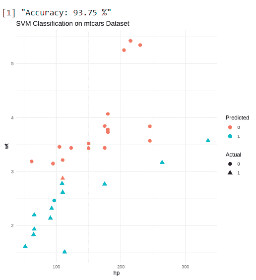
Output

You can download full code from here

Evaluation Metrics for Classification

When evaluating classification models, several metrics are used to measure performance. Each metric provides insights into different aspects of model accuracy and reliability.

1. Confusion Matrix

A confusion matrix is a table that describes the performance of a classification model by comparing actual vs predicted values. It shows:

• **True Positives (TP): Correctly predicted positive cases
• **True Negatives (TN): Correctly predicted negative cases
• **False Positives (FP): Incorrectly predicted positive cases
• **False Negatives (FN): Incorrectly predicted negative cases

2. Precision

Precision is the ratio of correctly predicted positive observations to the total predicted positives

Precision=\frac{TP}{TP+FP}

It measures how accurate the model is when it predicts the positive class.

3. Recall

Recall is the ratio of correctly predicted positive observations to all actual positives

Recall=\frac{TP}{TP+FN}

It measures the model’s ability to detect all actual positive cases.

4. F1-Score

The F1-Score is the weighted harmonic mean of Precision and Recall

F_1 = 2 \times \frac{\text{Precision} \times \text{Recall}}{\text{Precision} + \text{Recall}}

It provides a balance between precision and recall, especially useful when classes are imbalanced.