PieChart - Pie chart appearance and behavior - MATLAB (original) (raw)

PieChart Properties

Pie chart appearance and behavior

Since R2023b

PieChart properties control the appearance and behavior pie charts. By changing property values, you can modify certain aspects of these charts. Use dot notation to query and set properties.

p = piechart([1 2 3 4]); p.Names = ["Apple","Peach","Pizza","Pumpkin"];

Labels

expand all

Chart title, specified as a string vector, character vector, cell array of character vectors, or categorical array. To create a multiline title, specify a string vector or cell array of character vectors. Each element in the array is a separate line of text.

Alternatively, you can call the title function to add a title to the chart.

piechart([1 2 3 4]) title("My Pie Chart")

Slice labels, specified as a string vector or cell array of character vectors that has one value per slice.

Set this property if you want to change the labels that appear by default. The default labels might include the slice names depending on how you create your chart:

If you create the chart with numeric or duration data without specifying the slice names, MATLAB® assigns a default set of names to the Names property. However, the labels do not include those names. If you set theNames property explicitly, then the slice labels include the names.
If you create the chart with categorical data, then theNames property contains the category names, and the slice labels include those names.
If you create the chart with a table and specify a variable containing the names, then the Names property contains the names from that variable, and the slice labels include those names.

How the slices are labeled, specified as "auto" or"manual".

"auto" — Create and update the slice labels based on the Proportions and Names properties. If either of those properties change, the labels automatically update.
"manual" — Do not update the labels. When you set theLabels property, theLabelsMode property automatically changes to"manual".

Since R2024a

Label style, specified as one of the values in the table. When changing between different label styles, you might need to resize the figure to maintain the same size pie chart. Setting this property has no effect if the LabelsMode property is set to "manual".

Value	Description	Example
"namepercent"	Display the Names and Proportions values (as percentages) next to the corresponding slices.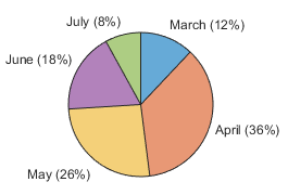
"namedata"	Display the Names and Data values next to the corresponding slices.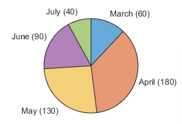
"name"	Display the Names values next to the corresponding slices.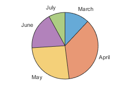
"data"	Display the Data values next to the corresponding slices.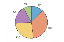
"percent"	Display the Proportions values (as percentages) next to the corresponding slices.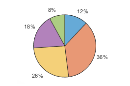
"none"	Do not display any labels.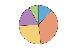

Since R2024a

How the label style is selected, specified as "auto" or"manual".

"auto" — MATLAB selects the label style based on your data (numeric or categorical) and the value of the NamesMode property.
"manual" — You specify the label style by setting theLabelStyle property.

Legend visibility, specified as "on" or "off", or as numeric or logical 1 (true) or0 (false). A value of "on" is equivalent to true, and "off" is equivalent tofalse. Thus, you can use the value of this property as a logical value. The value is stored as an on/off logical value of type matlab.lang.OnOffSwitchState.

When you set this property to "on", the legend is visible in the chart.

Legend title, specified as a string, character vector, cell array of character vectors, or categorical array. To create a multiline title, specify a string array or cell array of character vectors. Each element in the array is a separate line of text.

Text interpreter, specified as one of these values:

"tex" — Interpret characters using a subset of TeX markup.
"latex" — Interpret characters using LaTeX markup.
"none" — Display literal characters.

MATLAB uses the interpreter when displaying a chart title, axis labels, or any data that includes text or symbols.

TeX Markup

By default, MATLAB supports a subset of TeX markup. Use TeX markup to add superscripts and subscripts, modify the font type and color, and include special characters in the text.

Modifiers remain in effect until the end of the text. Superscripts and subscripts are an exception because they modify only the next character or the characters within the curly braces. When you set the interpreter to "tex", the supported modifiers are as follows.

Modifier	Description	Example
^{ }	Superscript	"text^{superscript}"
_{ }	Subscript	"text_{subscript}"
\bf	Bold font	"\bf text"
\it	Italic font	"\it text"
\sl	Oblique font (usually the same as italic font)	"\sl text"
\rm	Normal font	"\rm text"
\fontname{specifier}	Font name — Replace_specifier_ with the name of a font family. You can use this in combination with other modifiers.	"\fontname{Courier} text"
\fontsize{specifier}	Font size —Replace_specifier_ with a numeric scalar value in point units.	"\fontsize{15} text"
\color{specifier}	Font color — Replace_specifier_ with one of these colors: red, green,yellow, magenta,blue, black,white, gray,darkGreen, orange, orlightBlue.	"\color{magenta} text"
\color[rgb]{specifier}	Custom font color — Replace_specifier_ with a three-element RGB triplet.	"\color[rgb]{0,0.5,0.5} text"

This table lists the supported special characters for the"tex" interpreter.

Character Sequence	Symbol	Character Sequence	Symbol	Character Sequence	Symbol
\alpha	α	\upsilon	υ	\sim	~
\angle	∠	\phi	ϕ	\leq	≤
\ast	*	\chi	χ	\infty	∞
\beta	β	\psi	ψ	\clubsuit	♣
\gamma	γ	\omega	ω	\diamondsuit	♦
\delta	δ	\Gamma	Γ	\heartsuit	♥
\epsilon	ϵ	\Delta	Δ	\spadesuit	♠
\zeta	ζ	\Theta	Θ	\leftrightarrow	↔
\eta	η	\Lambda	Λ	\leftarrow	←
\theta	θ	\Xi	Ξ	\Leftarrow	⇐
\vartheta	ϑ	\Pi	Π	\uparrow	↑
\iota	ι	\Sigma	Σ	\rightarrow	→
\kappa	κ	\Upsilon	ϒ	\Rightarrow	⇒
\lambda	λ	\Phi	Φ	\downarrow	↓
\mu	µ	\Psi	Ψ	\circ	º
\nu	ν	\Omega	Ω	\pm	±
\xi	ξ	\forall	∀	\geq	≥
\pi	π	\exists	∃	\propto	∝
\rho	ρ	\ni	∍	\partial	∂
\sigma	σ	\cong	≅	\bullet	•
\varsigma	ς	\approx	≈	\div	÷
\tau	τ	\Re	ℜ	\neq	≠
\equiv	≡	\oplus	⊕	\aleph	ℵ
\Im	ℑ	\cup	∪	\wp	℘
\otimes	⊗	\subseteq	⊆	\oslash	∅
\cap	∩	\in	∈	\supseteq	⊇
\supset	⊃	\lceil	⌈	\subset	⊂
\int	∫	\cdot	·	\o	ο
\rfloor	⌋	\neg	¬	\nabla	∇
\lfloor	⌊	\times	x	\ldots	...
\perp	⊥	\surd	√	\prime	´
\wedge	∧	\varpi	ϖ	\0	∅
\rceil	⌉	\rangle	〉	\mid	\|
\vee	∨	\langle	〈	\copyright	©

LaTeX Markup

To use LaTeX markup, set the interpreter to "latex". For inline mode, surround the markup with single dollar signs ($). For display mode, surround the markup with double dollar signs ($$).

LaTeX Mode	Example	Result
Inline	"$\int_1^{20} x^2 dx$"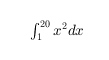
Display	"$$\int_1^{20} x^2 dx$$"

The displayed text uses the default LaTeX font style. To change the font style, use LaTeX markup.

The maximum size of the text that you can use with the LaTeX interpreter is 1200 characters. For multiline text, this reduces by about 10 characters per line.

MATLAB supports most standard LaTeX math mode commands. For more information, see Supported LaTeX Commands. For examples that use TeX and LaTeX, see Greek Letters and Special Characters in Chart Text.

Color and Styling

expand all

Color order, specified as a three-column matrix of RGB triplets. This property defines the palette of colors MATLAB uses to create the chart. Each row of the matrix is an RGB triplet. An RGB triplet is a three-element vector whose elements specify the intensities of the red, green, and blue components of a color. The intensities must be in the range [0, 1].

This table lists the default color palettes for plots in the light and dark themes.

Palette	Palette Colors
"gem" — Light theme default_Before R2025a: Most plots use these colors by default._
"glow" — Dark theme default

You can get the RGB triplets and hexadecimal color codes for these palettes using the orderedcolors and rgb2hex functions. For example, get the RGB triplets for the "gem" palette and convert them to hexadecimal color codes.

RGB = orderedcolors("gem"); H = rgb2hex(RGB);

Before R2023b: Get the RGB triplets using RGB = get(groot,"FactoryAxesColorOrder").

Before R2024a: Get the hexadecimal color codes using H = compose("#%02X%02X%02X",round(RGB*255)).

Note

You can set this property to one of several predefined color palettes by passing the PieChart object to the colororder function.

Slice colors, specified as a value from this table.

FaceColor Value	Description
"flat"	Let MATLAB assign a different color to each slice. The colors are defined in the ColorOrder property of the chart.
RGB triplet or hexadecimal color code	Assign one custom color to all the slices: RGB triplet — A three-element row vector whose elements specify the intensities of the red, green, and blue components of the color. The intensities must be in the range [0,1]; for example, [0.4 0.6 0.7].Hexadecimal color code — A character vector or a string scalar that starts with a hash symbol (#) followed by three or six hexadecimal digits, which can range from0 to F. The values are not case sensitive. Thus, the color codes"#FF8800","#ff8800","#F80", and"#f80" are equivalent.The two tables below provide the RGB triplets and hexadecimal color codes for some common colors.
Color name or short name	Assign one named color to all the slices using a color name such as "red", or a short name such as "r".The table below lists the available color names and short names.
"none"	Display all the slices without any color.

This table lists the available color names and short names with corresponding RGB triplets and hexadecimal color codes.

Color Name	Short Name	RGB Triplet	Hexadecimal Color Code
"red"	"r"	[1 0 0]	"#FF0000"
"green"	"g"	[0 1 0]	"#00FF00"
"blue"	"b"	[0 0 1]	"#0000FF"
"cyan"	"c"	[0 1 1]	"#00FFFF"
"magenta"	"m"	[1 0 1]	"#FF00FF"
"yellow"	"y"	[1 1 0]	"#FFFF00"
"black"	"k"	[0 0 0]	"#000000"
"white"	"w"	[1 1 1]	"#FFFFFF"

This table lists the default color palettes for plots in the light and dark themes.

Palette	Palette Colors
"gem" — Light theme default_Before R2025a: Most plots use these colors by default._
"glow" — Dark theme default

RGB = orderedcolors("gem"); H = rgb2hex(RGB);

Before R2023b: Get the RGB triplets using RGB = get(groot,"FactoryAxesColorOrder").

Before R2024a: Get the hexadecimal color codes using H = compose("#%02X%02X%02X",round(RGB*255)).

Slice outline color, specified as a value from this table.

EdgeColor Value	Description
"flat"	Let MATLAB assign a different outline color to each slice. The colors are defined in the ColorOrder property of the chart.
RGB triplet or hexadecimal color code	Assign one custom outline color to all the slices: RGB triplet — A three-element row vector whose elements specify the intensities of the red, green, and blue components of the color. The intensities must be in the range [0,1]; for example, [0.4 0.6 0.7].Hexadecimal color code — A character vector or a string scalar that starts with a hash symbol (#) followed by three or six hexadecimal digits, which can range from 0 to F. The values are not case sensitive. Thus, the color codes "#FF8800", "#ff8800", "#F80", and "#f80" are equivalent.The two tables below provide the RGB triplets and hexadecimal color codes for some common colors.
Color name or short name	Assign one named outline color to all the slices using a color name such as"red", or a short name such as"r".The table below lists the available color names and short names.
"none"	Display the chart without any outline color.

This table lists the available color names and short names with corresponding RGB triplets and hexadecimal color codes.

Color Name	Short Name	RGB Triplet	Hexadecimal Color Code
"red"	"r"	[1 0 0]	"#FF0000"
"green"	"g"	[0 1 0]	"#00FF00"
"blue"	"b"	[0 0 1]	"#0000FF"
"cyan"	"c"	[0 1 1]	"#00FFFF"
"magenta"	"m"	[1 0 1]	"#FF00FF"
"yellow"	"y"	[1 1 0]	"#FFFF00"
"black"	"k"	[0 0 0]	"#000000"
"white"	"w"	[1 1 1]	"#FFFFFF"

This table lists the default color palettes for plots in the light and dark themes.

Palette	Palette Colors
"gem" — Light theme default_Before R2025a: Most plots use these colors by default._
"glow" — Dark theme default

RGB = orderedcolors("gem"); H = rgb2hex(RGB);

Before R2023b: Get the RGB triplets using RGB = get(groot,"FactoryAxesColorOrder").

Before R2024a: Get the hexadecimal color codes using H = compose("#%02X%02X%02X",round(RGB*255)).

Slice fill color transparency, specified as a scalar in the range [0,1]. A value of 1 makes the slices opaque, and 0 makes them completely transparent. Values between 0 and1 make the slices partially transparent.

Thickness of slice outlines, specified as a positive value in points.

Offset slices, specified as a numeric or logical vector for numeric data. If you create the chart using categorical data, you can specify a string vector or a character vector containing one or more category names. The orange slice in this pie chart is offset.

Pie chart with the second slice offset

Example: piechart([5 7 4 6],ExplodedWedges=3) creates a pie chart with the third slice offset.

Example: piechart([5 7 4 6],ExplodedWedges=[1 3]) creates a pie chart with the first and third slice offset.

Example: piechart([5 7 4 6],ExplodedWedges=[false false true false]) creates a pie chart with the third slice offset.

Example: piechart(categorical(["A" "B" "C" "D"]),ExplodedWedges="B") creates a pie chart using categorical data with slice B offset.

Direction for adding slices, specified as "clockwise" or "counterclockwise".

"clockwise" — Add slices in a clockwise direction.
"counterclockwise" — Add slices in a counterclockwise direction.

Data Display

expand all

This property is read-only.

Category counts when you specify categorical data, returned as a numeric vector. The number of elements in the vector is the number of categories in your data. Each element of the vector contains the number of instances of a category.

Starting angle of the first slice, specified as a scalar value in degrees. By default, the starting angle is 0 degrees. Positive values rotate the slices in a clockwise direction. Negative values rotate the slices in a counterclockwise direction.

You can envision the location of the starting angle by considering the arrangement of numbers on a clock. A starting angle of 0 degrees corresponds to 12 o'clock, and a starting angle of 90 degrees corresponds to 3 o'clock.

Two pie charts with different starting angles. One chart has a starting angle of 0 degrees, and the other chart has a starting angle of 90 degrees.

This property is read-only.

Slice proportions, returned as a numeric vector containing the size of each slice as a proportion out of 1. If you create the chart using categorical data, then the proportions are the CategoryCounts divided by the number of categories.

Since R2024b

Slice display order, specified as one of the values in this table. By default, the first slice is positioned according to the StartAngle property, and subsequent slices follow clockwise or counterclockwise depending on theDirection property.

Value	Description	Example with Data=[3 2 4 1]
"data"	Order of the values in the Data property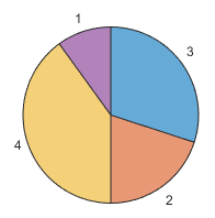
"ascend"	Ascending order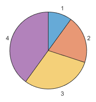
"descend"	Descending order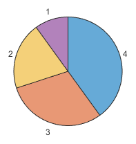

Since R2024b

Number of slices to display in the chart, specified as a positive whole number. By default, the chart displays all the data values using as many slices as needed. If you specify a number n that is less than Inf, and your data contains more than n values, the sum of the remaining values is displayed in an additional slice named "Others". To hide the"Others" slice, set the ShowOthers property to "off".

Since R2024b

Show the "Others" slice, specified as "on" or"off", or as numeric or logical 1 (true) or 0 (false). A value of "on" is equivalent to true, and"off" is equivalent to false. Thus, you can use the value of this property as a logical value. The value is stored as an on/off logical value of type matlab.lang.OnOffSwitchState.

"on" — If the NumDisplayWedges property is less than the number of values in the Data property, the chart displays an additional slice named"Others" that represents the sum of the remaining values. If you create the chart with a categorical array that contains<undefined> values, then the chart includes the<undefined> values in the "Others" slice.
"off" — Show only the number of slices specified byNumDisplayWedges. If NumDisplayWedges is Inf, show one slice for each data value that is not<undefined>.

Since R2024b

This property is read-only.

Data values of the displayed slices, returned as a numeric vector. The vector contains one element per slice in the order they appear in the chart.

Since R2024b

This property is read-only.

Names of the displayed slices, returned as a string vector. The vector contains one element per slice in the order they appear in the chart.

Font

expand all

Font size, specified as a scalar value greater than zero in point units. The default font size depends on the specific operating system and locale. One point equals1/72 inch.

How font size is selected, specified as "auto" or "manual".

"auto" — MATLAB selects the font size automatically and scales the text slightly according to the size of the chart, which typically changes when you resize the figure.
"manual" — You set the font size, and it remains unchanged regardless of the size of the chart.

Font color, specified as an RGB triplet, a hexadecimal color code, or one of the options listed in the table.

RGB triplets and hexadecimal color codes are useful for specifying custom colors.

An RGB triplet is a three-element row vector whose elements specify the intensities of the red, green, and blue components of the color. The intensities must be in the range [0,1]; for example, [0.4 0.6 0.7].
A hexadecimal color code is a character vector or a string scalar that starts with a hash symbol (#) followed by three or six hexadecimal digits, which can range from 0 to F. The values are not case sensitive. Thus, the color codes"#FF8800", "#ff8800","#F80", and "#f80" are equivalent.

Alternatively, you can specify some common colors by name. This table lists the named color options, the equivalent RGB triplets, and hexadecimal color codes.

Color Name	Short Name	RGB Triplet	Hexadecimal Color Code
"red"	"r"	[1 0 0]	"#FF0000"
"green"	"g"	[0 1 0]	"#00FF00"
"blue"	"b"	[0 0 1]	"#0000FF"
"cyan"	"c"	[0 1 1]	"#00FFFF"
"magenta"	"m"	[1 0 1]	"#FF00FF"
"yellow"	"y"	[1 1 0]	"#FFFF00"
"black"	"k"	[0 0 0]	"#000000"
"white"	"w"	[1 1 1]	"#FFFFFF"

This table lists the default color palettes for plots in the light and dark themes.

Palette	Palette Colors
"gem" — Light theme default_Before R2025a: Most plots use these colors by default._
"glow" — Dark theme default

RGB = orderedcolors("gem"); H = rgb2hex(RGB);

Before R2023b: Get the RGB triplets using RGB = get(groot,"FactoryAxesColorOrder").

Before R2024a: Get the hexadecimal color codes using H = compose("#%02X%02X%02X",round(RGB*255)).

Vector Data

expand all

Slice data, specified as a vector of numeric, duration, categorical, or logical values.

How the Data property is set, specified as one of these values:

"auto" — The Data property updates automatically based on the SourceTable andDataVariable properties. This is the case when you pass a table to the piechart ordonutchart functions.
"manual" — The Data property is set directly and does not update automatically. This is the case when you pass data values as a vector to the piechart ordonutchart functions.

Slice names, specified as a string vector or cell array of character vectors.

The default slice names, and whether you can change them, depend on how you create your chart:

If you create the chart with numeric or duration data without specifying the slice names, the Names property contains the string vector ["data1","data2",…,"dataN"]. However, the slice labels do not include those default names. If you set theNames property explicitly, then the slice labels include the names.
If you create the chart with categorical data, then theNames property contains the category names, and you cannot change them. In this case, the slice labels include the category names, and you can change the slice labels by setting the Labels property.
If you create the chart with a table and specify thenamesvar input argument, then theNames property contains the names from that table variable, and you cannot set the Names property directly. If you do not specify the namesvar argument when you create the chart, you can set the Names property.

How the Names property is set, specified as one of these values:

"auto" — MATLAB controls the value of the Names property. The Names value can be:
- The string vector["data1","data2",…,"dataN"] forN slices.
- A string vector of category names.
- The values in a table variable. TheSourceTable property specifies the table, and the NamesVariable property specifies the variable. If either theSourceTable orNamesVariableproperty is empty, then the Names property contains["data1","data2",…,"dataN"] instead.
"manual" — The Names property is set directly and does not update automatically. This is the case when you pass the slice names as a vector (such as a string or numeric vector) to thepiechart or donutchart functions.

Table Data

expand all

Source table containing the chart data. Specify this property as a table or a timetable.

Table variable containing the slice data, specified using one of the indexing schemes from the following table. The variable you specify can contain numeric, duration, categorical, or logical values. When you set this property, MATLAB updates the Data property. TheSourceTable property must contain a table with at least one variable. Otherwise, this property has no effect.

Indexing Scheme	Examples
Variable name:A string scalar or character vector.A pattern object. The pattern object must refer to only one variable.	"A" or 'A' — A variable named A"Var"+digitsPattern(1) — The variable with the name "Var" followed by a single digit
Variable index:An index number that refers to the location of a variable in the table.A logical vector. Typically, this vector is the same length as the number of variables, but you can omit trailing 0 or false values.	3 — The third variable from the table[false false true] — The third variable
Variable type:A vartype subscript that selects a table variable of a specified type. The subscript must refer to only one variable.	vartype("double") — The variable containing double values

Table variable containing the slice names, specified using one of the indexing schemes from the following table. The variable you specify can contain a string vector, a cell array of character vectors, or a vector of numeric, datetime, duration, or categorical values. When you set this property, MATLAB updates the Names property. TheSourceTable property must contain a table with at least one variable. Otherwise, this property has no effect.

Indexing Scheme	Examples
Variable name:A string scalar or character vector.A pattern object. The pattern object must refer to only one variable.	"A" or 'A' — A variable named A"Var"+digitsPattern(1) — The variable with the name "Var" followed by a single digit
Variable index:An index number that refers to the location of a variable in the table.A logical vector. Typically, this vector is the same length as the number of variables, but you can omit trailing 0 or false values.	3 — The third variable from the table[false false true] — The third variable
Variable type:A vartype subscript that selects a table variable of a specified type. The subscript must refer to only one variable.	vartype("double") — The variable containing double values

Position

expand all

Outer size and location of the chart within the parent container (typically a figure, panel, or tiled chart layout), specified as a four-element vector of the form[left bottom width height]. The outer size and location includes the legend and title.

The left and bottom elements define the distance from the lower-left corner of the container to the lower-left corner of the chart.
The width and height elements are the chart dimensions, which include a margin for the surrounding legend and title.

The default value of [0 0 1 1] covers the whole interior of the container. The units are normalized relative to the size of the container. To change the units, set the Units property.

Note

Setting this property has no effect when the parent container is aTiledChartLayout object.

Inner size and location of the chart within the parent container (typically a figure, panel, or tiled chart layout) specified as a four-element vector of the form[left bottom width height]. The inner size and location does not include the legend or title.

The left and bottom elements define the distance from the lower-left corner of the container to the lower-left corner of the box that encloses the chart.
The width and height elements are the dimensions of the box that encloses the chart.

Note

Setting this property has no effect when the parent container is aTiledChartLayout object.

Inner size and location of the chart within the parent container (typically a figure, panel, or tiled chart layout), specified as a four-element vector of the form[left bottom width height]. This property is equivalent to theInnerPosition property.

Note

Setting this property has no effect when the parent container is aTiledChartLayout object.

Position property to hold constant when adding, removing, or changing decorations, specified as one of the following values:

"outerposition" — TheOuterPosition property remains constant when you add, remove, or change decorations such as a title or an axis label. If any positional adjustments are needed, MATLAB adjusts the InnerPosition property.
"innerposition" — TheInnerPosition property remains constant when you add, remove, or change decorations such as a title or an axis label. If any positional adjustments are needed, MATLAB adjusts the OuterPosition property.

Note

Setting this property has no effect when the parent container is aTiledChartLayout object.

Position units, specified as one of the values in this table.

Units	Description
"normalized" (default)	Normalized with respect to the container, which is typically the figure or a panel. The lower-left corner of the container maps to(0,0), and the upper-right corner maps to(1,1).
"inches"	Inches.
"centimeters"	Centimeters.
"characters"	Based on the default font of the graphics root object: Character width = width of letter x.Character height = distance between the baselines of two lines of text.
"points"	Typography points. One point equals 1/72 inch.
"pixels"	Pixels.On Windows® and Macintosh systems, the size of a pixel is 1/96th of an inch. This size is independent of your system resolution.On Linux® systems, the size of a pixel is determined by your system resolution.

When specifying the units as a name-value pair during object creation, you must set the Units property before specifying the properties that you want to use these units, such as OuterPosition.

Layout options, specified as a TiledChartLayoutOptions orGridLayoutOptions object. This property is useful when the chart is either in a tiled chart layout or a grid layout.

To position the chart within the grid of a tiled chart layout, set theTile and TileSpan properties on theTiledChartLayoutOptions object. For example, consider a 3-by-3 tiled chart layout. The layout has a grid of tiles in the center, and four tiles along the outer edges. In practice, the grid is invisible and the outer tiles do not take up space until you populate them with axes or charts.

Diagram of a 3-by-3 tiled chart layout.

This code places the chart c in the third tile of the grid.

To make the chart span multiple tiles, specify the TileSpan property as a two-element vector. For example, this chart spans 2 rows and 3 columns of tiles.

c.Layout.TileSpan = [2 3];

To place the chart in one of the surrounding tiles, specify theTile property as "north","south", "east", or "west". For example, setting the value to "east" places the chart in the tile to the right of the grid.

To place the chart into a layout within an app, specify this property as aGridLayoutOptions object. For more information about working with grid layouts in apps, see uigridlayout.

If the chart is not a child of either a tiled chart layout or a grid layout (for example, if it is a child of a figure or panel) then this property is empty and has no effect.

State of visibility, specified as "on" or"off", or as numeric or logical 1 (true) or 0 (false). A value of "on" is equivalent to true, and"off" is equivalent to false. Thus, you can use the value of this property as a logical value. The value is stored as an on/off logical value of type matlab.lang.OnOffSwitchState.

"on" — Display the chart.
"off" — Hide the chart without deleting it. You still can access the properties of an invisible PieChart object.

Parent/Child

expand all

Parent container, specified as a Figure,Panel, Tab,TiledChartLayout, or GridLayout object.

Version History

Introduced in R2023b

expand all

Use LaTeX or TeX markup in the titles and labels of your chart by setting theInterpreter property of the PieChart object to"latex" or "tex". To display text without an interpreter, set this property to "none".

Simplify pie charts with large numbers of slices by setting properties that control the order and number of slices. Use the property DisplayOrder to arrange slices from largest to smallest and use the NumDisplayWedges property to specify the number of slices to display separately (the remaining slice data is grouped together as a slice labeled "Others").

Other useful properties include:

ShowOthers — Show a slice labeled "Others" to represent values not shown as individual slices. For example,<undefined> categorical values are represented in the"Others" slice.
WedgeDisplayNames — Return the labels of the slices shown in the chart.
WedgeDisplayData — Return the data values for slices shown in the chart.

You can specify different slice labels by setting the LabelStyle property.