Version 0.14.0 (May 31 , 2014) — pandas 3.0.0.dev0+2099.g3832e85779 documentation (original) (raw)

This is a major release from 0.13.1 and includes a small number of API changes, several new features, enhancements, and performance improvements along with a large number of bug fixes. We recommend that all users upgrade to this version.

• Highlights include:
  • Officially support Python 3.4
  • SQL interfaces updated to use sqlalchemy, See Here.
  • Display interface changes, See Here
  • MultiIndexing Using Slicers, See Here.
  • Ability to join a singly-indexed DataFrame with a MultiIndexed DataFrame, see Here
  • More consistency in groupby results and more flexible groupby specifications, See Here
  • Holiday calendars are now supported in CustomBusinessDay, see Here
  • Several improvements in plotting functions, including: hexbin, area and pie plots, see Here.
  • Performance doc section on I/O operations, See Here
• Other Enhancements
• API Changes
• Text Parsing API Changes
• Groupby API Changes
• Performance Improvements
• Prior Deprecations
• Deprecations
• Known Issues
• Bug Fixes

Warning

In 0.14.0 all NDFrame based containers have undergone significant internal refactoring. Before that each block of homogeneous data had its own labels and extra care was necessary to keep those in sync with the parent container’s labels. This should not have any visible user/API behavior changes (GH 6745)

API changes#

• read_excel uses 0 as the default sheet (GH 6573)
• iloc will now accept out-of-bounds indexers for slices, e.g. a value that exceeds the length of the object being indexed. These will be excluded. This will make pandas conform more with python/numpy indexing of out-of-bounds values. A single indexer that is out-of-bounds and drops the dimensions of the object will still raiseIndexError (GH 6296, GH 6299). This could result in an empty axis (e.g. an empty DataFrame being returned)
  In [1]: dfl = pd.DataFrame(np.random.randn(5, 2), columns=list('AB'))
  In [2]: dfl
  Out[2]:
  A B

0 0.469112 -0.282863
1 -1.509059 -1.135632
2 1.212112 -0.173215
3 0.119209 -1.044236
4 -0.861849 -2.104569
[5 rows x 2 columns]
In [3]: dfl.iloc[:, 2:3]
Out[3]:
Empty DataFrame
Columns: []
Index: [0, 1, 2, 3, 4]
[5 rows x 0 columns]
In [4]: dfl.iloc[:, 1:3]
Out[4]:
B
0 -0.282863
1 -1.135632
2 -0.173215
3 -1.044236
4 -2.104569
[5 rows x 1 columns]
In [5]: dfl.iloc[4:6]
Out[5]:
A B
4 -0.861849 -2.104569
[1 rows x 2 columns]
These are out-of-bounds selections

dfl.iloc[[4, 5, 6]]
IndexError: positional indexers are out-of-bounds
dfl.iloc[:, 4]
IndexError: single positional indexer is out-of-bounds

• Slicing with negative start, stop & step values handles corner cases better (GH 6531):
  • df.iloc[:-len(df)] is now empty
  • df.iloc[len(df)::-1] now enumerates all elements in reverse
• The DataFrame.interpolate() keyword downcast default has been changed from infer toNone. This is to preserve the original dtype unless explicitly requested otherwise (GH 6290).
• When converting a dataframe to HTML it used to return Empty DataFrame. This special case has been removed, instead a header with the column names is returned (GH 6062).
• Series and Index now internally share more common operations, e.g. factorize(),nunique(),value_counts() are now supported on Index types as well. The Series.weekday property from is removed from Series for API consistency. Using a DatetimeIndex/PeriodIndex method on a Series will now raise a TypeError. (GH 4551, GH 4056, GH 5519, GH 6380, GH 7206).
• Add is_month_start, is_month_end, is_quarter_start, is_quarter_end, is_year_start, is_year_end accessors for DateTimeIndex / Timestamp which return a boolean array of whether the timestamp(s) are at the start/end of the month/quarter/year defined by the frequency of the DateTimeIndex / Timestamp (GH 4565, GH 6998)
• Local variable usage has changed inpandas.eval()/DataFrame.eval()/DataFrame.query()(GH 5987). For the DataFrame methods, two things have changed
  • Column names are now given precedence over locals
  • Local variables must be referred to explicitly. This means that even if you have a local variable that is not a column you must still refer to it with the '@' prefix.
  • You can have an expression like df.query('@a < a') with no complaints from pandas about ambiguity of the name a.
  • The top-level pandas.eval() function does not allow you use the'@' prefix and provides you with an error message telling you so.
  • NameResolutionError was removed because it isn’t necessary anymore.
• Define and document the order of column vs index names in query/eval (GH 6676)
• concat will now concatenate mixed Series and DataFrames using the Series name or numbering columns as needed (GH 2385). See the docs
• Slicing and advanced/boolean indexing operations on Index classes as well as Index.delete() and Index.drop() methods will no longer change the type of the resulting index (GH 6440, GH 7040)
  In [6]: i = pd.Index([1, 2, 3, 'a', 'b', 'c'])
  In [7]: i[[0, 1, 2]]
  Out[7]: Index([1, 2, 3], dtype='object')
  In [8]: i.drop(['a', 'b', 'c'])
  Out[8]: Index([1, 2, 3], dtype='object')
  Previously, the above operation would return Int64Index. If you’d like to do this manually, use Index.astype()
  In [9]: i[[0, 1, 2]].astype(np.int_)
  Out[9]: Index([1, 2, 3], dtype='int64')
• set_index no longer converts MultiIndexes to an Index of tuples. For example, the old behavior returned an Index in this case (GH 6459):

Old behavior, casted MultiIndex to an Index

In [10]: tuple_ind
Out[10]: Index([('a', 'c'), ('a', 'd'), ('b', 'c'), ('b', 'd')], dtype='object')
In [11]: df_multi.set_index(tuple_ind)
Out[11]:
0 1
(a, c) 0.471435 -1.190976
(a, d) 1.432707 -0.312652
(b, c) -0.720589 0.887163
(b, d) 0.859588 -0.636524
[4 rows x 2 columns]

New behavior

In [12]: mi
Out[12]:
MultiIndex([('a', 'c'),
('a', 'd'),
('b', 'c'),
('b', 'd')],
)
In [13]: df_multi.set_index(mi)
Out[13]:
0 1
a c 0.471435 -1.190976
d 1.432707 -0.312652
b c -0.720589 0.887163
d 0.859588 -0.636524
[4 rows x 2 columns]
This also applies when passing multiple indices to set_index:

Old output, 2-level MultiIndex of tuples

In [14]: df_multi.set_index([df_multi.index, df_multi.index])
Out[14]:
0 1
(a, c) (a, c) 0.471435 -1.190976
(a, d) (a, d) 1.432707 -0.312652
(b, c) (b, c) -0.720589 0.887163
(b, d) (b, d) 0.859588 -0.636524
[4 rows x 2 columns]

New output, 4-level MultiIndex

In [15]: df_multi.set_index([df_multi.index, df_multi.index])
Out[15]:
0 1
a c a c 0.471435 -1.190976
d a d 1.432707 -0.312652
b c b c -0.720589 0.887163
d b d 0.859588 -0.636524
[4 rows x 2 columns]

• pairwise keyword was added to the statistical moment functionsrolling_cov, rolling_corr, ewmcov, ewmcorr,expanding_cov, expanding_corr to allow the calculation of moving window covariance and correlation matrices (GH 4950). SeeComputing rolling pairwise covariances and correlations in the docs.
  In [1]: df = pd.DataFrame(np.random.randn(10, 4), columns=list('ABCD'))
  In [4]: covs = pd.rolling_cov(df[['A', 'B', 'C']],
  ....: df[['B', 'C', 'D']],
  ....: 5,
  ....: pairwise=True)
  In [5]: covs[df.index[-1]]
  Out[5]:
  B C D

A 0.035310 0.326593 -0.505430
B 0.137748 -0.006888 -0.005383
C -0.006888 0.861040 0.020762

• Series.iteritems() is now lazy (returns an iterator rather than a list). This was the documented behavior prior to 0.14. (GH 6760)
• Added nunique and value_counts functions to Index for counting unique elements. (GH 6734)
• stack and unstack now raise a ValueError when the level keyword refers to a non-unique item in the Index (previously raised a KeyError). (GH 6738)
• drop unused order argument from Series.sort; args now are in the same order as Series.order; add na_position arg to conform to Series.order (GH 6847)
• default sorting algorithm for Series.order is now quicksort, to conform with Series.sort(and numpy defaults)
• add inplace keyword to Series.order/sort to make them inverses (GH 6859)
• DataFrame.sort now places NaNs at the beginning or end of the sort according to the na_position parameter. (GH 3917)
• accept TextFileReader in concat, which was affecting a common user idiom (GH 6583), this was a regression from 0.13.1
• Added factorize functions to Index and Series to get indexer and unique values (GH 7090)
• describe on a DataFrame with a mix of Timestamp and string like objects returns a different Index (GH 7088). Previously the index was unintentionally sorted.
• Arithmetic operations with only bool dtypes now give a warning indicating that they are evaluated in Python space for +, -, and * operations and raise for all others (GH 7011, GH 6762,GH 7015, GH 7210)

  x = pd.Series(np.random.rand(10) > 0.5)
  y = True
  x + y # warning generated: should do x | y instead
  UserWarning: evaluating in Python space because the '+' operator is not
  supported by numexpr for the bool dtype, use '|' instead
  x / y # this raises because it doesn't make sense
  NotImplementedError: operator '/' not implemented for bool dtypes

• In HDFStore, select_as_multiple will always raise a KeyError, when a key or the selector is not found (GH 6177)
• df['col'] = value and df.loc[:,'col'] = value are now completely equivalent; previously the .loc would not necessarily coerce the dtype of the resultant series (GH 6149)
• dtypes and ftypes now return a series with dtype=object on empty containers (GH 5740)
• df.to_csv will now return a string of the CSV data if neither a target path nor a buffer is provided (GH 6061)
• pd.infer_freq() will now raise a TypeError if given an invalid Series/Indextype (GH 6407, GH 6463)
• A tuple passed to DataFame.sort_index will be interpreted as the levels of the index, rather than requiring a list of tuple (GH 4370)
• all offset operations now return Timestamp types (rather than datetime), Business/Week frequencies were incorrect (GH 4069)
• to_excel now converts np.inf into a string representation, customizable by the inf_rep keyword argument (Excel has no native inf representation) (GH 6782)
• Replace pandas.compat.scipy.scoreatpercentile with numpy.percentile (GH 6810)
• .quantile on a datetime[ns] series now returns Timestamp instead of np.datetime64 objects (GH 6810)
• change AssertionError to TypeError for invalid types passed to concat (GH 6583)
• Raise a TypeError when DataFrame is passed an iterator as thedata argument (GH 5357)

Display changes#

• The default way of printing large DataFrames has changed. DataFrames exceeding max_rows and/or max_columns are now displayed in a centrally truncated view, consistent with the printing of apandas.Series (GH 5603).
  In previous versions, a DataFrame was truncated once the dimension constraints were reached and an ellipse (…) signaled that part of the data was cut off.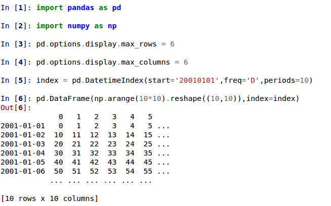
  
  In the current version, large DataFrames are centrally truncated, showing a preview of head and tail in both dimensions.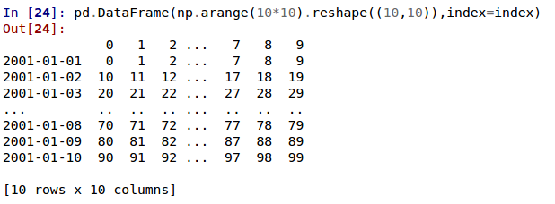
  
• allow option 'truncate' for display.show_dimensions to only show the dimensions if the frame is truncated (GH 6547).
  The default for display.show_dimensions will now be truncate. This is consistent with how Series display length.
  In [16]: dfd = pd.DataFrame(np.arange(25).reshape(-1, 5),
  ....: index=[0, 1, 2, 3, 4],
  ....: columns=[0, 1, 2, 3, 4])
  ....:

show dimensions since this is truncated

In [17]: with pd.option_context('display.max_rows', 2, 'display.max_columns', 2,
....: 'display.show_dimensions', 'truncate'):
....: print(dfd)
....:
0 ... 4
0 0 ... 4
.. .. ... ..
4 20 ... 24
[5 rows x 5 columns]

will not show dimensions since it is not truncated

In [18]: with pd.option_context('display.max_rows', 10, 'display.max_columns', 40,
....: 'display.show_dimensions', 'truncate'):
....: print(dfd)
....:
0 1 2 3 4
0 0 1 2 3 4
1 5 6 7 8 9
2 10 11 12 13 14
3 15 16 17 18 19
4 20 21 22 23 24

• Regression in the display of a MultiIndexed Series with display.max_rows is less than the length of the series (GH 7101)
• Fixed a bug in the HTML repr of a truncated Series or DataFrame not showing the class name with thelarge_repr set to ‘info’ (GH 7105)
• The verbose keyword in DataFrame.info(), which controls whether to shorten the inforepresentation, is now None by default. This will follow the global setting indisplay.max_info_columns. The global setting can be overridden with verbose=True orverbose=False.
• Fixed a bug with the info repr not honoring the display.max_info_columns setting (GH 6939)
• Offset/freq info now in Timestamp __repr__ (GH 4553)

Text parsing API changes#

read_csv()/read_table() will now be noisier w.r.t invalid options rather than falling back to the PythonParser.

• Raise ValueError when sep specified withdelim_whitespace=True in read_csv()/read_table()(GH 6607)
• Raise ValueError when engine='c' specified with unsupported options in read_csv()/read_table() (GH 6607)
• Raise ValueError when fallback to python parser causes options to be ignored (GH 6607)
• Produce ParserWarning on fallback to python parser when no options are ignored (GH 6607)
• Translate sep='\s+' to delim_whitespace=True inread_csv()/read_table() if no other C-unsupported options specified (GH 6607)

GroupBy API changes#

More consistent behavior for some groupby methods:

• groupby head and tail now act more like filter rather than an aggregation:
  In [1]: df = pd.DataFrame([[1, 2], [1, 4], [5, 6]], columns=['A', 'B'])
  In [2]: g = df.groupby('A')
  In [3]: g.head(1) # filters DataFrame
  Out[3]:
  A B
  0 1 2
  2 5 6
  In [4]: g.apply(lambda x: x.head(1)) # used to simply fall-through
  Out[4]:
  A B
  A
  1 0 1 2
  5 2 5 6
• groupby head and tail respect column selection:
  In [19]: g[['B']].head(1)
  Out[19]:
  B
  0 2
  2 6
  [2 rows x 1 columns]
• groupby nth now reduces by default; filtering can be achieved by passing as_index=False. With an optional dropna argument to ignore NaN. See the docs.
  Reducing
  In [19]: df = pd.DataFrame([[1, np.nan], [1, 4], [5, 6]], columns=['A', 'B'])
  In [20]: g = df.groupby('A')
  In [21]: g.nth(0)
  Out[21]:
  A B
  0 1 NaN
  2 5 6.0
  [2 rows x 2 columns]

this is equivalent to g.first()

In [22]: g.nth(0, dropna='any')
Out[22]:
A B
1 1 4.0
2 5 6.0
[2 rows x 2 columns]

this is equivalent to g.last()

In [23]: g.nth(-1, dropna='any')
Out[23]:
A B
1 1 4.0
2 5 6.0
[2 rows x 2 columns]
Filtering
In [24]: gf = df.groupby('A', as_index=False)
In [25]: gf.nth(0)
Out[25]:
A B
0 1 NaN
2 5 6.0
[2 rows x 2 columns]
In [26]: gf.nth(0, dropna='any')
Out[26]:
A B
1 1 4.0
2 5 6.0
[2 rows x 2 columns]

• groupby will now not return the grouped column for non-cython functions (GH 5610, GH 5614, GH 6732), as its already the index
  In [27]: df = pd.DataFrame([[1, np.nan], [1, 4], [5, 6], [5, 8]], columns=['A', 'B'])
  In [28]: g = df.groupby('A')
  In [29]: g.count()
  Out[29]:
  B
  A
  1 1
  5 2
  [2 rows x 1 columns]
  In [30]: g.describe()
  Out[30]:
  B
  count mean std min 25% 50% 75% max
  A
  1 1.0 4.0 NaN 4.0 4.0 4.0 4.0 4.0
  5 2.0 7.0 1.414214 6.0 6.5 7.0 7.5 8.0
  [2 rows x 8 columns]
• passing as_index will leave the grouped column in-place (this is not change in 0.14.0)
  In [31]: df = pd.DataFrame([[1, np.nan], [1, 4], [5, 6], [5, 8]], columns=['A', 'B'])
  In [32]: g = df.groupby('A', as_index=False)
  In [33]: g.count()
  Out[33]:
  A B
  0 1 1
  1 5 2
  [2 rows x 2 columns]
  In [34]: g.describe()
  Out[34]:
  A B
  count mean std min 25% 50% 75% max
  0 1 1.0 4.0 NaN 4.0 4.0 4.0 4.0 4.0
  1 5 2.0 7.0 1.414214 6.0 6.5 7.0 7.5 8.0
  [2 rows x 9 columns]
• Allow specification of a more complex groupby via pd.Grouper, such as grouping by a Time and a string field simultaneously. See the docs. (GH 3794)
• Better propagation/preservation of Series names when performing groupby operations:
  • SeriesGroupBy.agg will ensure that the name attribute of the original series is propagated to the result (GH 6265).
  • If the function provided to GroupBy.apply returns a named series, the name of the series will be kept as the name of the column index of the DataFrame returned by GroupBy.apply (GH 6124). This facilitatesDataFrame.stack operations where the name of the column index is used as the name of the inserted column containing the pivoted data.

SQL#

The SQL reading and writing functions now support more database flavors through SQLAlchemy (GH 2717, GH 4163, GH 5950, GH 6292). All databases supported by SQLAlchemy can be used, such as PostgreSQL, MySQL, Oracle, Microsoft SQL server (see documentation of SQLAlchemy on included dialects).

The functionality of providing DBAPI connection objects will only be supported for sqlite3 in the future. The 'mysql' flavor is deprecated.

The new functions read_sql_query() and read_sql_table()are introduced. The function read_sql() is kept as a convenience wrapper around the other two and will delegate to specific function depending on the provided input (database table name or sql query).

In practice, you have to provide a SQLAlchemy engine to the sql functions. To connect with SQLAlchemy you use the create_engine() function to create an engine object from database URI. You only need to create the engine once per database you are connecting to. For an in-memory sqlite database:

In [35]: from sqlalchemy import create_engine

Create your connection.

In [36]: engine = create_engine('sqlite:///:memory:')

This engine can then be used to write or read data to/from this database:

In [37]: df = pd.DataFrame({'A': [1, 2, 3], 'B': ['a', 'b', 'c']})

In [38]: df.to_sql(name='db_table', con=engine, index=False) Out[38]: 3

You can read data from a database by specifying the table name:

In [39]: pd.read_sql_table('db_table', engine) Out[39]: A B 0 1 a 1 2 b 2 3 c

[3 rows x 2 columns]

or by specifying a sql query:

In [40]: pd.read_sql_query('SELECT * FROM db_table', engine) Out[40]: A B 0 1 a 1 2 b 2 3 c

[3 rows x 2 columns]

Some other enhancements to the sql functions include:

• support for writing the index. This can be controlled with the indexkeyword (default is True).
• specify the column label to use when writing the index with index_label.
• specify string columns to parse as datetimes with the parse_dateskeyword in read_sql_query() and read_sql_table().

Warning

Some of the existing functions or function aliases have been deprecated and will be removed in future versions. This includes: tquery, uquery,read_frame, frame_query, write_frame.

Warning

The support for the ‘mysql’ flavor when using DBAPI connection objects has been deprecated. MySQL will be further supported with SQLAlchemy engines (GH 6900).

Multi-indexing using slicers#

In 0.14.0 we added a new way to slice MultiIndexed objects. You can slice a MultiIndex by providing multiple indexers.

You can provide any of the selectors as if you are indexing by label, see Selection by Label, including slices, lists of labels, labels, and boolean indexers.

You can use slice(None) to select all the contents of that level. You do not need to specify all the_deeper_ levels, they will be implied as slice(None).

As usual, both sides of the slicers are included as this is label indexing.

See the docsSee also issues (GH 6134, GH 4036, GH 3057, GH 2598, GH 5641, GH 7106)

Warning

You should specify all axes in the .loc specifier, meaning the indexer for the index and for the columns. Their are some ambiguous cases where the passed indexer could be mis-interpreted as indexing both axes, rather than into say the MultiIndex for the rows.

You should do this:

df.loc[(slice('A1', 'A3'), ...), :] # noqa: E901

rather than this:

df.loc[(slice('A1', 'A3'), ...)] # noqa: E901

Warning

You will need to make sure that the selection axes are fully lexsorted!

In [41]: def mklbl(prefix, n): ....: return ["%s%s" % (prefix, i) for i in range(n)] ....:

In [42]: index = pd.MultiIndex.from_product([mklbl('A', 4), ....: mklbl('B', 2), ....: mklbl('C', 4), ....: mklbl('D', 2)]) ....:

In [43]: columns = pd.MultiIndex.from_tuples([('a', 'foo'), ('a', 'bar'), ....: ('b', 'foo'), ('b', 'bah')], ....: names=['lvl0', 'lvl1']) ....:

In [44]: df = pd.DataFrame(np.arange(len(index) * len(columns)).reshape((len(index), ....: len(columns))), ....: index=index, ....: columns=columns).sort_index().sort_index(axis=1) ....:

In [45]: df Out[45]: lvl0 a b
lvl1 bar foo bah foo A0 B0 C0 D0 1 0 3 2 D1 5 4 7 6 C1 D0 9 8 11 10 D1 13 12 15 14 C2 D0 17 16 19 18 ... ... ... ... ... A3 B1 C1 D1 237 236 239 238 C2 D0 241 240 243 242 D1 245 244 247 246 C3 D0 249 248 251 250 D1 253 252 255 254

[64 rows x 4 columns]

Basic MultiIndex slicing using slices, lists, and labels.

In [46]: df.loc[(slice('A1', 'A3'), slice(None), ['C1', 'C3']), :] Out[46]: lvl0 a b
lvl1 bar foo bah foo A1 B0 C1 D0 73 72 75 74 D1 77 76 79 78 C3 D0 89 88 91 90 D1 93 92 95 94 B1 C1 D0 105 104 107 106 ... ... ... ... ... A3 B0 C3 D1 221 220 223 222 B1 C1 D0 233 232 235 234 D1 237 236 239 238 C3 D0 249 248 251 250 D1 253 252 255 254

[24 rows x 4 columns]

You can use a pd.IndexSlice to shortcut the creation of these slices

In [47]: idx = pd.IndexSlice

In [48]: df.loc[idx[:, :, ['C1', 'C3']], idx[:, 'foo']] Out[48]: lvl0 a b lvl1 foo foo A0 B0 C1 D0 8 10 D1 12 14 C3 D0 24 26 D1 28 30 B1 C1 D0 40 42 ... ... ... A3 B0 C3 D1 220 222 B1 C1 D0 232 234 D1 236 238 C3 D0 248 250 D1 252 254

[32 rows x 2 columns]

It is possible to perform quite complicated selections using this method on multiple axes at the same time.

In [49]: df.loc['A1', (slice(None), 'foo')] Out[49]: lvl0 a b lvl1 foo foo B0 C0 D0 64 66 D1 68 70 C1 D0 72 74 D1 76 78 C2 D0 80 82 ... ... ... B1 C1 D1 108 110 C2 D0 112 114 D1 116 118 C3 D0 120 122 D1 124 126

[16 rows x 2 columns]

In [50]: df.loc[idx[:, :, ['C1', 'C3']], idx[:, 'foo']] Out[50]: lvl0 a b lvl1 foo foo A0 B0 C1 D0 8 10 D1 12 14 C3 D0 24 26 D1 28 30 B1 C1 D0 40 42 ... ... ... A3 B0 C3 D1 220 222 B1 C1 D0 232 234 D1 236 238 C3 D0 248 250 D1 252 254

[32 rows x 2 columns]

Using a boolean indexer you can provide selection related to the values.

In [51]: mask = df[('a', 'foo')] > 200

In [52]: df.loc[idx[mask, :, ['C1', 'C3']], idx[:, 'foo']] Out[52]: lvl0 a b lvl1 foo foo A3 B0 C1 D1 204 206 C3 D0 216 218 D1 220 222 B1 C1 D0 232 234 D1 236 238 C3 D0 248 250 D1 252 254

[7 rows x 2 columns]

You can also specify the axis argument to .loc to interpret the passed slicers on a single axis.

In [53]: df.loc(axis=0)[:, :, ['C1', 'C3']] Out[53]: lvl0 a b
lvl1 bar foo bah foo A0 B0 C1 D0 9 8 11 10 D1 13 12 15 14 C3 D0 25 24 27 26 D1 29 28 31 30 B1 C1 D0 41 40 43 42 ... ... ... ... ... A3 B0 C3 D1 221 220 223 222 B1 C1 D0 233 232 235 234 D1 237 236 239 238 C3 D0 249 248 251 250 D1 253 252 255 254

[32 rows x 4 columns]

Furthermore you can set the values using these methods

In [54]: df2 = df.copy()

In [55]: df2.loc(axis=0)[:, :, ['C1', 'C3']] = -10

In [56]: df2 Out[56]: lvl0 a b
lvl1 bar foo bah foo A0 B0 C0 D0 1 0 3 2 D1 5 4 7 6 C1 D0 -10 -10 -10 -10 D1 -10 -10 -10 -10 C2 D0 17 16 19 18 ... ... ... ... ... A3 B1 C1 D1 -10 -10 -10 -10 C2 D0 241 240 243 242 D1 245 244 247 246 C3 D0 -10 -10 -10 -10 D1 -10 -10 -10 -10

[64 rows x 4 columns]

You can use a right-hand-side of an alignable object as well.

In [57]: df2 = df.copy()

In [58]: df2.loc[idx[:, :, ['C1', 'C3']], :] = df2 * 1000

In [59]: df2 Out[59]: lvl0 a b
lvl1 bar foo bah foo A0 B0 C0 D0 1 0 3 2 D1 5 4 7 6 C1 D0 9000 8000 11000 10000 D1 13000 12000 15000 14000 C2 D0 17 16 19 18 ... ... ... ... ... A3 B1 C1 D1 237000 236000 239000 238000 C2 D0 241 240 243 242 D1 245 244 247 246 C3 D0 249000 248000 251000 250000 D1 253000 252000 255000 254000

[64 rows x 4 columns]

Plotting#

• Hexagonal bin plots from DataFrame.plot with kind='hexbin' (GH 5478), See the docs.
• DataFrame.plot and Series.plot now supports area plot with specifying kind='area' (GH 6656), See the docs
• Pie plots from Series.plot and DataFrame.plot with kind='pie' (GH 6976), See the docs.
• Plotting with Error Bars is now supported in the .plot method of DataFrame and Series objects (GH 3796, GH 6834), See the docs.
• DataFrame.plot and Series.plot now support a table keyword for plotting matplotlib.Table, See the docs. The table keyword can receive the following values.
  • False: Do nothing (default).
  • True: Draw a table using the DataFrame or Series called plot method. Data will be transposed to meet matplotlib’s default layout.
  • DataFrame or Series: Draw matplotlib.table using the passed data. The data will be drawn as displayed in print method (not transposed automatically). Also, helper function pandas.tools.plotting.table is added to create a table from DataFrame and Series, and add it to an matplotlib.Axes.
• plot(legend='reverse') will now reverse the order of legend labels for most plot kinds. (GH 6014)
• Line plot and area plot can be stacked by stacked=True (GH 6656)
• Following keywords are now acceptable for DataFrame.plot() with kind='bar' and kind='barh':
  • width: Specify the bar width. In previous versions, static value 0.5 was passed to matplotlib and it cannot be overwritten. (GH 6604)
  • align: Specify the bar alignment. Default is center (different from matplotlib). In previous versions, pandas passes align='edge' to matplotlib and adjust the location to center by itself, and it results align keyword is not applied as expected. (GH 4525)
  • position: Specify relative alignments for bar plot layout. From 0 (left/bottom-end) to 1(right/top-end). Default is 0.5 (center). (GH 6604)
    Because of the default align value changes, coordinates of bar plots are now located on integer values (0.0, 1.0, 2.0 …). This is intended to make bar plot be located on the same coordinates as line plot. However, bar plot may differs unexpectedly when you manually adjust the bar location or drawing area, such as using set_xlim, set_ylim, etc. In this cases, please modify your script to meet with new coordinates.
• The parallel_coordinates() function now takes argument colorinstead of colors. A FutureWarning is raised to alert that the old colors argument will not be supported in a future release. (GH 6956)
• The parallel_coordinates() and andrews_curves() functions now take positional argument frame instead of data. A FutureWarning is raised if the old data argument is used by name. (GH 6956)
• DataFrame.boxplot() now supports layout keyword (GH 6769)
• DataFrame.boxplot() has a new keyword argument, return_type. It accepts 'dict','axes', or 'both', in which case a namedtuple with the matplotlib axes and a dict of matplotlib Lines is returned.

Prior version deprecations/changes#

There are prior version deprecations that are taking effect as of 0.14.0.

• Remove DateRange in favor of DatetimeIndex (GH 6816)
• Remove column keyword from DataFrame.sort (GH 4370)
• Remove precision keyword from set_eng_float_format() (GH 395)
• Remove force_unicode keyword from DataFrame.to_string(),DataFrame.to_latex(), and DataFrame.to_html(); these function encode in unicode by default (GH 2224, GH 2225)
• Remove nanRep keyword from DataFrame.to_csv() andDataFrame.to_string() (GH 275)
• Remove unique keyword from HDFStore.select_column() (GH 3256)
• Remove inferTimeRule keyword from Timestamp.offset() (GH 391)
• Remove name keyword from get_data_yahoo() andget_data_google() ( commit b921d1a )
• Remove offset keyword from DatetimeIndex constructor ( commit 3136390 )
• Remove time_rule from several rolling-moment statistical functions, such as rolling_sum() (GH 1042)
• Removed neg - boolean operations on numpy arrays in favor of inv ~, as this is going to be deprecated in numpy 1.9 (GH 6960)

Deprecations#

• The pivot_table()/DataFrame.pivot_table() and crosstab() functions now take arguments index and columns instead of rows and cols. AFutureWarning is raised to alert that the old rows and cols arguments will not be supported in a future release (GH 5505)
• The DataFrame.drop_duplicates() and DataFrame.duplicated() methods now take argument subset instead of cols to better align withDataFrame.dropna(). A FutureWarning is raised to alert that the oldcols arguments will not be supported in a future release (GH 6680)
• The DataFrame.to_csv() and DataFrame.to_excel() functions now takes argument columns instead of cols. AFutureWarning is raised to alert that the old cols arguments will not be supported in a future release (GH 6645)
• Indexers will warn FutureWarning when used with a scalar indexer and a non-floating point Index (GH 4892, GH 6960)

non-floating point indexes can only be indexed by integers / labels

In [1]: pd.Series(1, np.arange(5))[3.0]
pandas/core/index.py:469: FutureWarning: scalar indexers for index type Int64Index should be integers and not floating point
Out[1]: 1
In [2]: pd.Series(1, np.arange(5)).iloc[3.0]
pandas/core/index.py:469: FutureWarning: scalar indexers for index type Int64Index should be integers and not floating point
Out[2]: 1
In [3]: pd.Series(1, np.arange(5)).iloc[3.0:4]
pandas/core/index.py:527: FutureWarning: slice indexers when using iloc should be integers and not floating point
Out[3]:
3 1
dtype: int64

these are Float64Indexes, so integer or floating point is acceptable

In [4]: pd.Series(1, np.arange(5.))[3]
Out[4]: 1
In [5]: pd.Series(1, np.arange(5.))[3.0]
Out[6]: 1

• Numpy 1.9 compat w.r.t. deprecation warnings (GH 6960)
• Panel.shift() now has a function signature that matches DataFrame.shift(). The old positional argument lags has been changed to a keyword argumentperiods with a default value of 1. A FutureWarning is raised if the old argument lags is used by name. (GH 6910)
• The order keyword argument of factorize() will be removed. (GH 6926).
• Remove the copy keyword from DataFrame.xs(), Panel.major_xs(), Panel.minor_xs(). A view will be returned if possible, otherwise a copy will be made. Previously the user could think that copy=False would ALWAYS return a view. (GH 6894)
• The parallel_coordinates() function now takes argument colorinstead of colors. A FutureWarning is raised to alert that the old colors argument will not be supported in a future release. (GH 6956)
• The parallel_coordinates() and andrews_curves() functions now take positional argument frame instead of data. A FutureWarning is raised if the old data argument is used by name. (GH 6956)
• The support for the ‘mysql’ flavor when using DBAPI connection objects has been deprecated. MySQL will be further supported with SQLAlchemy engines (GH 6900).
• The following io.sql functions have been deprecated: tquery, uquery, read_frame, frame_query, write_frame.
• The percentile_width keyword argument in describe() has been deprecated. Use the percentiles keyword instead, which takes a list of percentiles to display. The default output is unchanged.
• The default return type of boxplot() will change from a dict to a matplotlib Axes in a future release. You can use the future behavior now by passing return_type='axes'to boxplot.

Known issues#

• OpenPyXL 2.0.0 breaks backwards compatibility (GH 7169)

Enhancements#

• DataFrame and Series will create a MultiIndex object if passed a tuples dict, See the docs (GH 3323)
  In [60]: pd.Series({('a', 'b'): 1, ('a', 'a'): 0,
  ....: ('a', 'c'): 2, ('b', 'a'): 3, ('b', 'b'): 4})
  ....:
  Out[60]:
  a b 1
  a 0
  c 2
  b a 3
  b 4
  Length: 5, dtype: int64
  In [61]: pd.DataFrame({('a', 'b'): {('A', 'B'): 1, ('A', 'C'): 2},
  ....: ('a', 'a'): {('A', 'C'): 3, ('A', 'B'): 4},
  ....: ('a', 'c'): {('A', 'B'): 5, ('A', 'C'): 6},
  ....: ('b', 'a'): {('A', 'C'): 7, ('A', 'B'): 8},
  ....: ('b', 'b'): {('A', 'D'): 9, ('A', 'B'): 10}})
  ....:
  Out[61]:
  a b
  b a c a b

A B 1.0 4.0 5.0 8.0 10.0
C 2.0 3.0 6.0 7.0 NaN
D NaN NaN NaN NaN 9.0
[3 rows x 5 columns]

• Added the sym_diff method to Index (GH 5543)
• DataFrame.to_latex now takes a longtable keyword, which if True will return a table in a longtable environment. (GH 6617)
• Add option to turn off escaping in DataFrame.to_latex (GH 6472)
• pd.read_clipboard will, if the keyword sep is unspecified, try to detect data copied from a spreadsheet and parse accordingly. (GH 6223)
• Joining a singly-indexed DataFrame with a MultiIndexed DataFrame (GH 3662)
  See the docs. Joining MultiIndex DataFrames on both the left and right is not yet supported ATM.
  In [62]: household = pd.DataFrame({'household_id': [1, 2, 3],
  ....: 'male': [0, 1, 0],
  ....: 'wealth': [196087.3, 316478.7, 294750]
  ....: },
  ....: columns=['household_id', 'male', 'wealth']
  ....: ).set_index('household_id')
  ....:
  In [63]: household
  Out[63]:
  male wealth

household_id
1 0 196087.3
2 1 316478.7
3 0 294750.0
[3 rows x 2 columns]
In [64]: portfolio = pd.DataFrame({'household_id': [1, 2, 2, 3, 3, 3, 4],
....: 'asset_id': ["nl0000301109",
....: "nl0000289783",
....: "gb00b03mlx29",
....: "gb00b03mlx29",
....: "lu0197800237",
....: "nl0000289965",
....: np.nan],
....: 'name': ["ABN Amro",
....: "Robeco",
....: "Royal Dutch Shell",
....: "Royal Dutch Shell",
....: "AAB Eastern Europe Equity Fund",
....: "Postbank BioTech Fonds",
....: np.nan],
....: 'share': [1.0, 0.4, 0.6, 0.15, 0.6, 0.25, 1.0]
....: },
....: columns=['household_id', 'asset_id', 'name', 'share']
....: ).set_index(['household_id', 'asset_id'])
....:
In [65]: portfolio
Out[65]:
name share
household_id asset_id
1 nl0000301109 ABN Amro 1.00
2 nl0000289783 Robeco 0.40
gb00b03mlx29 Royal Dutch Shell 0.60
3 gb00b03mlx29 Royal Dutch Shell 0.15
lu0197800237 AAB Eastern Europe Equity Fund 0.60
nl0000289965 Postbank BioTech Fonds 0.25
4 NaN NaN 1.00
[7 rows x 2 columns]
In [66]: household.join(portfolio, how='inner')
Out[66]:
male ... share
household_id asset_id ...
1 nl0000301109 0 ... 1.00
2 nl0000289783 1 ... 0.40
gb00b03mlx29 1 ... 0.60
3 gb00b03mlx29 0 ... 0.15
lu0197800237 0 ... 0.60
nl0000289965 0 ... 0.25
[6 rows x 4 columns]

• quotechar, doublequote, and escapechar can now be specified when using DataFrame.to_csv (GH 5414, GH 4528)
• Partially sort by only the specified levels of a MultiIndex with thesort_remaining boolean kwarg. (GH 3984)
• Added to_julian_date to TimeStamp and DatetimeIndex. The Julian Date is used primarily in astronomy and represents the number of days from noon, January 1, 4713 BC. Because nanoseconds are used to define the time in pandas the actual range of dates that you can use is 1678 AD to 2262 AD. (GH 4041)
• DataFrame.to_stata will now check data for compatibility with Stata data types and will upcast when needed. When it is not possible to losslessly upcast, a warning is issued (GH 6327)
• DataFrame.to_stata and StataWriter will accept keyword arguments time_stamp and data_label which allow the time stamp and dataset label to be set when creating a file. (GH 6545)
• pandas.io.gbq now handles reading unicode strings properly. (GH 5940)
• Holidays Calendars are now available and can be used with the CustomBusinessDay offset (GH 6719)
• Float64Index is now backed by a float64 dtype ndarray instead of anobject dtype array (GH 6471).
• Implemented Panel.pct_change (GH 6904)
• Added how option to rolling-moment functions to dictate how to handle resampling; rolling_max() defaults to max,rolling_min() defaults to min, and all others default to mean (GH 6297)
• CustomBusinessMonthBegin and CustomBusinessMonthEnd are now available (GH 6866)
• Series.quantile() and DataFrame.quantile() now accept an array of quantiles.
• describe() now accepts an array of percentiles to include in the summary statistics (GH 4196)
• pivot_table can now accept Grouper by index and columns keywords (GH 6913)
  In [67]: import datetime
  In [68]: df = pd.DataFrame({
  ....: 'Branch': 'A A A A A B'.split(),
  ....: 'Buyer': 'Carl Mark Carl Carl Joe Joe'.split(),
  ....: 'Quantity': [1, 3, 5, 1, 8, 1],
  ....: 'Date': [datetime.datetime(2013, 11, 1, 13, 0),
  ....: datetime.datetime(2013, 9, 1, 13, 5),
  ....: datetime.datetime(2013, 10, 1, 20, 0),
  ....: datetime.datetime(2013, 10, 2, 10, 0),
  ....: datetime.datetime(2013, 11, 1, 20, 0),
  ....: datetime.datetime(2013, 10, 2, 10, 0)],
  ....: 'PayDay': [datetime.datetime(2013, 10, 4, 0, 0),
  ....: datetime.datetime(2013, 10, 15, 13, 5),
  ....: datetime.datetime(2013, 9, 5, 20, 0),
  ....: datetime.datetime(2013, 11, 2, 10, 0),
  ....: datetime.datetime(2013, 10, 7, 20, 0),
  ....: datetime.datetime(2013, 9, 5, 10, 0)]})
  ....:
  In [69]: df
  Out[69]:
  Branch Buyer Quantity Date PayDay
  0 A Carl 1 2013-11-01 13:00:00 2013-10-04 00:00:00

1 A Mark 3 2013-09-01 13:05:00 2013-10-15 13:05:00
2 A Carl 5 2013-10-01 20:00:00 2013-09-05 20:00:00
3 A Carl 1 2013-10-02 10:00:00 2013-11-02 10:00:00
4 A Joe 8 2013-11-01 20:00:00 2013-10-07 20:00:00
5 B Joe 1 2013-10-02 10:00:00 2013-09-05 10:00:00
[6 rows x 5 columns]
In [75]: df.pivot_table(values='Quantity',
....: index=pd.Grouper(freq='M', key='Date'),
....: columns=pd.Grouper(freq='M', key='PayDay'),
....: aggfunc="sum")
Out[75]:
PayDay 2013-09-30 2013-10-31 2013-11-30
Date
2013-09-30 NaN 3.0 NaN
2013-10-31 6.0 NaN 1.0
2013-11-30 NaN 9.0 NaN
[3 rows x 3 columns]

• Arrays of strings can be wrapped to a specified width (str.wrap) (GH 6999)
• Add nsmallest() and Series.nlargest() methods to Series, See the docs (GH 3960)
• PeriodIndex fully supports partial string indexing like DatetimeIndex (GH 7043)
  In [76]: prng = pd.period_range('2013-01-01 09:00', periods=100, freq='H')
  In [77]: ps = pd.Series(np.random.randn(len(prng)), index=prng)
  In [78]: ps
  Out[78]:
  2013-01-01 09:00 0.015696
  2013-01-01 10:00 -2.242685
  2013-01-01 11:00 1.150036
  2013-01-01 12:00 0.991946
  2013-01-01 13:00 0.953324
  ...

2013-01-05 08:00 0.285296
2013-01-05 09:00 0.484288
2013-01-05 10:00 1.363482
2013-01-05 11:00 -0.781105
2013-01-05 12:00 -0.468018
Freq: H, Length: 100, dtype: float64
In [79]: ps['2013-01-02']
Out[79]:
2013-01-02 00:00 0.553439
2013-01-02 01:00 1.318152
2013-01-02 02:00 -0.469305
2013-01-02 03:00 0.675554
2013-01-02 04:00 -1.817027
...
2013-01-02 19:00 0.036142
2013-01-02 20:00 -2.074978
2013-01-02 21:00 0.247792
2013-01-02 22:00 -0.897157
2013-01-02 23:00 -0.136795
Freq: H, Length: 24, dtype: float64

• read_excel can now read milliseconds in Excel dates and times with xlrd >= 0.9.3. (GH 5945)
• pd.stats.moments.rolling_var now uses Welford’s method for increased numerical stability (GH 6817)
• pd.expanding_apply and pd.rolling_apply now take args and kwargs that are passed on to the func (GH 6289)
• DataFrame.rank() now has a percentage rank option (GH 5971)
• Series.rank() now has a percentage rank option (GH 5971)
• Series.rank() and DataFrame.rank() now accept method='dense' for ranks without gaps (GH 6514)
• Support passing encoding with xlwt (GH 3710)
• Refactor Block classes removing Block.items attributes to avoid duplication in item handling (GH 6745, GH 6988).
• Testing statements updated to use specialized asserts (GH 6175)

Performance#

• Performance improvement when converting DatetimeIndex to floating ordinals using DatetimeConverter (GH 6636)
• Performance improvement for DataFrame.shift (GH 5609)
• Performance improvement in indexing into a MultiIndexed Series (GH 5567)
• Performance improvements in single-dtyped indexing (GH 6484)
• Improve performance of DataFrame construction with certain offsets, by removing faulty caching (e.g. MonthEnd,BusinessMonthEnd), (GH 6479)
• Improve performance of CustomBusinessDay (GH 6584)
• improve performance of slice indexing on Series with string keys (GH 6341, GH 6372)
• Performance improvement for DataFrame.from_records when reading a specified number of rows from an iterable (GH 6700)
• Performance improvements in timedelta conversions for integer dtypes (GH 6754)
• Improved performance of compatible pickles (GH 6899)
• Improve performance in certain reindexing operations by optimizing take_2d (GH 6749)
• GroupBy.count() is now implemented in Cython and is much faster for large numbers of groups (GH 7016).

Experimental#

There are no experimental changes in 0.14.0

Bug fixes#

• Bug in Series ValueError when index doesn’t match data (GH 6532)
• Prevent segfault due to MultiIndex not being supported in HDFStore table format (GH 1848)
• Bug in pd.DataFrame.sort_index where mergesort wasn’t stable when ascending=False (GH 6399)
• Bug in pd.tseries.frequencies.to_offset when argument has leading zeros (GH 6391)
• Bug in version string gen. for dev versions with shallow clones / install from tarball (GH 6127)
• Inconsistent tz parsing Timestamp / to_datetime for current year (GH 5958)
• Indexing bugs with reordered indexes (GH 6252, GH 6254)
• Bug in .xs with a Series multiindex (GH 6258, GH 5684)
• Bug in conversion of a string types to a DatetimeIndex with a specified frequency (GH 6273, GH 6274)
• Bug in eval where type-promotion failed for large expressions (GH 6205)
• Bug in interpolate with inplace=True (GH 6281)
• HDFStore.remove now handles start and stop (GH 6177)
• HDFStore.select_as_multiple handles start and stop the same way as select (GH 6177)
• HDFStore.select_as_coordinates and select_column works with a where clause that results in filters (GH 6177)
• Regression in join of non_unique_indexes (GH 6329)
• Issue with groupby agg with a single function and a mixed-type frame (GH 6337)
• Bug in DataFrame.replace() when passing a non- bool to_replace argument (GH 6332)
• Raise when trying to align on different levels of a MultiIndex assignment (GH 3738)
• Bug in setting complex dtypes via boolean indexing (GH 6345)
• Bug in TimeGrouper/resample when presented with a non-monotonic DatetimeIndex that would return invalid results. (GH 4161)
• Bug in index name propagation in TimeGrouper/resample (GH 4161)
• TimeGrouper has a more compatible API to the rest of the groupers (e.g. groups was missing) (GH 3881)
• Bug in multiple grouping with a TimeGrouper depending on target column order (GH 6764)
• Bug in pd.eval when parsing strings with possible tokens like '&'(GH 6351)
• Bug correctly handle placements of -inf in Panels when dividing by integer 0 (GH 6178)
• DataFrame.shift with axis=1 was raising (GH 6371)
• Disabled clipboard tests until release time (run locally with nosetests -A disabled) (GH 6048).
• Bug in DataFrame.replace() when passing a nested dict that contained keys not in the values to be replaced (GH 6342)
• str.match ignored the na flag (GH 6609).
• Bug in take with duplicate columns that were not consolidated (GH 6240)
• Bug in interpolate changing dtypes (GH 6290)
• Bug in Series.get, was using a buggy access method (GH 6383)
• Bug in hdfstore queries of the form where=[('date', '>=', datetime(2013,1,1)), ('date', '<=', datetime(2014,1,1))] (GH 6313)
• Bug in DataFrame.dropna with duplicate indices (GH 6355)
• Regression in chained getitem indexing with embedded list-like from 0.12 (GH 6394)
• Float64Index with nans not comparing correctly (GH 6401)
• eval/query expressions with strings containing the @ character will now work (GH 6366).
• Bug in Series.reindex when specifying a method with some nan values was inconsistent (noted on a resample) (GH 6418)
• Bug in DataFrame.replace() where nested dicts were erroneously depending on the order of dictionary keys and values (GH 5338).
• Performance issue in concatenating with empty objects (GH 3259)
• Clarify sorting of sym_diff on Index objects with NaN values (GH 6444)
• Regression in MultiIndex.from_product with a DatetimeIndex as input (GH 6439)
• Bug in str.extract when passed a non-default index (GH 6348)
• Bug in str.split when passed pat=None and n=1 (GH 6466)
• Bug in io.data.DataReader when passed "F-F_Momentum_Factor" and data_source="famafrench" (GH 6460)
• Bug in sum of a timedelta64[ns] series (GH 6462)
• Bug in resample with a timezone and certain offsets (GH 6397)
• Bug in iat/iloc with duplicate indices on a Series (GH 6493)
• Bug in read_html where nan’s were incorrectly being used to indicate missing values in text. Should use the empty string for consistency with the rest of pandas (GH 5129).
• Bug in read_html tests where redirected invalid URLs would make one test fail (GH 6445).
• Bug in multi-axis indexing using .loc on non-unique indices (GH 6504)
• Bug that caused _ref_locs corruption when slice indexing across columns axis of a DataFrame (GH 6525)
• Regression from 0.13 in the treatment of numpy datetime64 non-ns dtypes in Series creation (GH 6529)
• .names attribute of MultiIndexes passed to set_index are now preserved (GH 6459).
• Bug in setitem with a duplicate index and an alignable rhs (GH 6541)
• Bug in setitem with .loc on mixed integer Indexes (GH 6546)
• Bug in pd.read_stata which would use the wrong data types and missing values (GH 6327)
• Bug in DataFrame.to_stata that lead to data loss in certain cases, and could be exported using the wrong data types and missing values (GH 6335)
• StataWriter replaces missing values in string columns by empty string (GH 6802)
• Inconsistent types in Timestamp addition/subtraction (GH 6543)
• Bug in preserving frequency across Timestamp addition/subtraction (GH 4547)
• Bug in empty list lookup caused IndexError exceptions (GH 6536, GH 6551)
• Series.quantile raising on an object dtype (GH 6555)
• Bug in .xs with a nan in level when dropped (GH 6574)
• Bug in fillna with method='bfill/ffill' and datetime64[ns] dtype (GH 6587)
• Bug in sql writing with mixed dtypes possibly leading to data loss (GH 6509)
• Bug in Series.pop (GH 6600)
• Bug in iloc indexing when positional indexer matched Int64Index of the corresponding axis and no reordering happened (GH 6612)
• Bug in fillna with limit and value specified
• Bug in DataFrame.to_stata when columns have non-string names (GH 4558)
• Bug in compat with np.compress, surfaced in (GH 6658)
• Bug in binary operations with a rhs of a Series not aligning (GH 6681)
• Bug in DataFrame.to_stata which incorrectly handles nan values and ignores with_index keyword argument (GH 6685)
• Bug in resample with extra bins when using an evenly divisible frequency (GH 4076)
• Bug in consistency of groupby aggregation when passing a custom function (GH 6715)
• Bug in resample when how=None resample freq is the same as the axis frequency (GH 5955)
• Bug in downcasting inference with empty arrays (GH 6733)
• Bug in obj.blocks on sparse containers dropping all but the last items of same for dtype (GH 6748)
• Bug in unpickling NaT (NaTType) (GH 4606)
• Bug in DataFrame.replace() where regex meta characters were being treated as regex even when regex=False (GH 6777).
• Bug in timedelta ops on 32-bit platforms (GH 6808)
• Bug in setting a tz-aware index directly via .index (GH 6785)
• Bug in expressions.py where numexpr would try to evaluate arithmetic ops (GH 6762).
• Bug in Makefile where it didn’t remove Cython generated C files with make clean (GH 6768)
• Bug with numpy < 1.7.2 when reading long strings from HDFStore (GH 6166)
• Bug in DataFrame._reduce where non bool-like (0/1) integers were being converted into bools. (GH 6806)
• Regression from 0.13 with fillna and a Series on datetime-like (GH 6344)
• Bug in adding np.timedelta64 to DatetimeIndex with timezone outputs incorrect results (GH 6818)
• Bug in DataFrame.replace() where changing a dtype through replacement would only replace the first occurrence of a value (GH 6689)
• Better error message when passing a frequency of ‘MS’ in Period construction (GH5332)
• Bug in Series.__unicode__ when max_rows=None and the Series has more than 1000 rows. (GH 6863)
• Bug in groupby.get_group where a datelike wasn’t always accepted (GH 5267)
• Bug in groupBy.get_group created by TimeGrouper raises AttributeError (GH 6914)
• Bug in DatetimeIndex.tz_localize and DatetimeIndex.tz_convert converting NaT incorrectly (GH 5546)
• Bug in arithmetic operations affecting NaT (GH 6873)
• Bug in Series.str.extract where the resulting Series from a single group match wasn’t renamed to the group name
• Bug in DataFrame.to_csv where setting index=False ignored theheader kwarg (GH 6186)
• Bug in DataFrame.plot and Series.plot, where the legend behave inconsistently when plotting to the same axes repeatedly (GH 6678)
• Internal tests for patching __finalize__ / bug in merge not finalizing (GH 6923, GH 6927)
• accept TextFileReader in concat, which was affecting a common user idiom (GH 6583)
• Bug in C parser with leading white space (GH 3374)
• Bug in C parser with delim_whitespace=True and \r-delimited lines
• Bug in python parser with explicit MultiIndex in row following column header (GH 6893)
• Bug in Series.rank and DataFrame.rank that caused small floats (<1e-13) to all receive the same rank (GH 6886)
• Bug in DataFrame.apply with functions that used *args or **kwargs and returned an empty result (GH 6952)
• Bug in sum/mean on 32-bit platforms on overflows (GH 6915)
• Moved Panel.shift to NDFrame.slice_shift and fixed to respect multiple dtypes. (GH 6959)
• Bug in enabling subplots=True in DataFrame.plot only has single column raises TypeError, and Series.plot raises AttributeError (GH 6951)
• Bug in DataFrame.plot draws unnecessary axes when enabling subplots and kind=scatter (GH 6951)
• Bug in read_csv from a filesystem with non-utf-8 encoding (GH 6807)
• Bug in iloc when setting / aligning (GH 6766)
• Bug causing UnicodeEncodeError when get_dummies called with unicode values and a prefix (GH 6885)
• Bug in timeseries-with-frequency plot cursor display (GH 5453)
• Bug surfaced in groupby.plot when using a Float64Index (GH 7025)
• Stopped tests from failing if options data isn’t able to be downloaded from Yahoo (GH 7034)
• Bug in parallel_coordinates and radviz where reordering of class column caused possible color/class mismatch (GH 6956)
• Bug in radviz and andrews_curves where multiple values of ‘color’ were being passed to plotting method (GH 6956)
• Bug in Float64Index.isin() where containing nan s would make indices claim that they contained all the things (GH 7066).
• Bug in DataFrame.boxplot where it failed to use the axis passed as the ax argument (GH 3578)
• Bug in the XlsxWriter and XlwtWriter implementations that resulted in datetime columns being formatted without the time (GH 7075) were being passed to plotting method
• read_fwf() treats None in colspec like regular python slices. It now reads from the beginning or until the end of the line when colspec contains a None (previously raised a TypeError)
• Bug in cache coherence with chained indexing and slicing; add _is_view property to NDFrame to correctly predict views; mark is_copy on xs only if its an actual copy (and not a view) (GH 7084)
• Bug in DatetimeIndex creation from string ndarray with dayfirst=True (GH 5917)
• Bug in MultiIndex.from_arrays created from DatetimeIndex doesn’t preserve freq and tz (GH 7090)
• Bug in unstack raises ValueError when MultiIndex contains PeriodIndex (GH 4342)
• Bug in boxplot and hist draws unnecessary axes (GH 6769)
• Regression in groupby.nth() for out-of-bounds indexers (GH 6621)
• Bug in quantile with datetime values (GH 6965)
• Bug in Dataframe.set_index, reindex and pivot don’t preserve DatetimeIndex and PeriodIndex attributes (GH 3950, GH 5878, GH 6631)
• Bug in MultiIndex.get_level_values doesn’t preserve DatetimeIndex and PeriodIndex attributes (GH 7092)
• Bug in Groupby doesn’t preserve tz (GH 3950)
• Bug in PeriodIndex partial string slicing (GH 6716)
• Bug in the HTML repr of a truncated Series or DataFrame not showing the class name with the large_repr set to ‘info’ (GH 7105)
• Bug in DatetimeIndex specifying freq raises ValueError when passed value is too short (GH 7098)
• Fixed a bug with the info repr not honoring the display.max_info_columns setting (GH 6939)
• Bug PeriodIndex string slicing with out of bounds values (GH 5407)
• Fixed a memory error in the hashtable implementation/factorizer on resizing of large tables (GH 7157)
• Bug in isnull when applied to 0-dimensional object arrays (GH 7176)
• Bug in query/eval where global constants were not looked up correctly (GH 7178)
• Bug in recognizing out-of-bounds positional list indexers with iloc and a multi-axis tuple indexer (GH 7189)
• Bug in setitem with a single value, MultiIndex and integer indices (GH 7190, GH 7218)
• Bug in expressions evaluation with reversed ops, showing in series-dataframe ops (GH 7198, GH 7192)
• Bug in multi-axis indexing with > 2 ndim and a MultiIndex (GH 7199)
• Fix a bug where invalid eval/query operations would blow the stack (GH 5198)

Contributors#

A total of 94 people contributed patches to this release. People with a “+” by their names contributed a patch for the first time.

• Acanthostega +
• Adam Marcus +
• Alex Gaudio
• Alex Rothberg
• AllenDowney +
• Andrew Rosenfeld +
• Andy Hayden
• Antoine Mazières +
• Benedikt Sauer
• Brad Buran
• Christopher Whelan
• Clark Fitzgerald
• DSM
• Dale Jung
• Dan Allan
• Dan Birken
• Daniel Waeber
• David Jung +
• David Stephens +
• Douglas McNeil
• Garrett Drapala
• Gouthaman Balaraman +
• Guillaume Poulin +
• Jacob Howard +
• Jacob Schaer
• Jason Sexauer +
• Jeff Reback
• Jeff Tratner
• Jeffrey Starr +
• John David Reaver +
• John McNamara
• John W. O’Brien
• Jonathan Chambers
• Joris Van den Bossche
• Julia Evans
• Júlio +
• K.-Michael Aye
• Katie Atkinson +
• Kelsey Jordahl
• Kevin Sheppard +
• Matt Wittmann +
• Matthias Kuhn +
• Max Grender-Jones +
• Michael E. Gruen +
• Mike Kelly
• Nipun Batra +
• Noah Spies +
• PKEuS
• Patrick O’Keeffe
• Phillip Cloud
• Pietro Battiston +
• Randy Carnevale +
• Robert Gibboni +
• Skipper Seabold
• SplashDance +
• Stephan Hoyer +
• Tim Cera +
• Tobias Brandt
• Todd Jennings +
• Tom Augspurger
• TomAugspurger
• Yaroslav Halchenko
• agijsberts +
• akittredge
• ankostis +
• anomrake
• anton-d +
• bashtage +
• benjamin +
• bwignall
• cgohlke +
• chebee7i +
• clham +
• danielballan
• hshimizu77 +
• hugo +
• immerrr
• ischwabacher +
• jaimefrio +
• jreback
• jsexauer +
• kdiether +
• michaelws +
• mikebailey +
• ojdo +
• onesandzeroes +
• phaebz +
• ribonoous +
• rockg
• sinhrks +
• unutbu
• westurner
• y-p
• zach powers