layout - Change layout of graph plot - MATLAB (original) (raw)
Change layout of graph plot
Syntax
Description
layout([H](#buxdj61%5Fsep%5Fshared-H)) changes the layout of graph plot H by using an automatic choice of layout method based on the structure of the graph. The layout function modifies theXData and YData properties ofH.
layout([H](#buxdj61%5Fsep%5Fshared-H),[method](#buxdj61-method)) optionally specifies the layout method. method can be'circle', 'force','layered', 'subspace','force3', or 'subspace3'.
layout([H](#buxdj61%5Fsep%5Fshared-H),[method](#buxdj61-method),[Name,Value](#namevaluepairarguments)) uses additional options specified by one or more name-value pair arguments. For example, layout(H,'force','Iterations',N) specifies the number of iterations to use in computing the force layout, andlayout(H,'layered','Sources',S) uses a layered layout with source nodes S included in the first layer.
Examples
Graph Layout Based on Structure
Create and plot a graph using the 'force' layout.
s = [1 1 1 1 1 6 6 6 6 6]; t = [2 3 4 5 6 7 8 9 10 11]; G = graph(s,t); h = plot(G,'Layout','force');
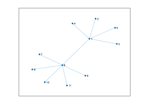
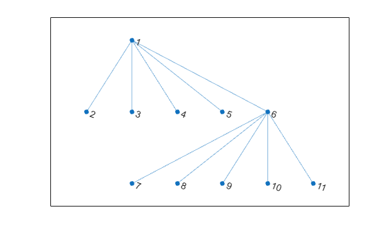
Change the layout to be the default that plot determines based on the structure and properties of the graph. The result is the same as using plot(G).
Change Layout of Graph
Create and plot a graph using the 'layered' layout.
s = [1 1 1 2 2 3 3 4 5 5 6 7]; t = [2 4 5 3 6 4 7 8 6 8 7 8]; G = graph(s,t); h = plot(G,'Layout','layered');
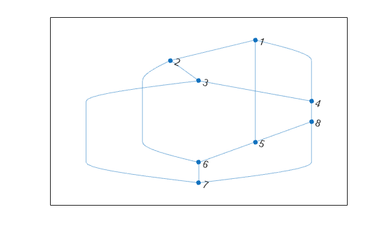
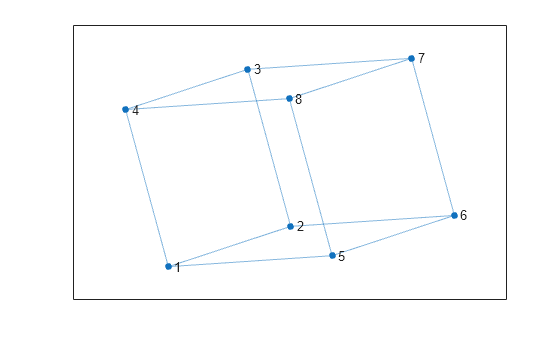
Change the layout of the graph to use the 'subspace' method.
Refine Layout Method of Graph
Create and plot a graph using the 'layered' layout method.
s = [1 1 1 2 3 3 3 4 4]; t = [2 4 5 6 2 4 7 8 1]; G = digraph(s,t); h = plot(G,'Layout','layered');
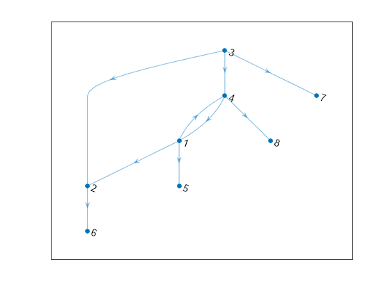
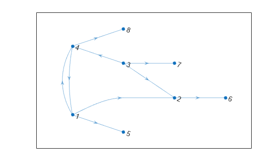
Use the layout function to refine the hierarchical layout by specifying source nodes and a horizontal orientation.
layout(h,'layered','Direction','right','Sources',[1 4])
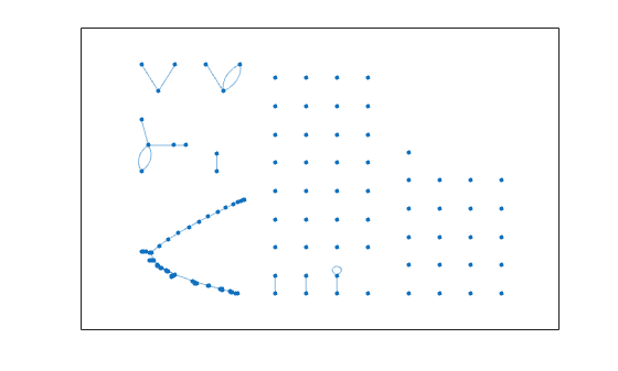
Graph Layout with Multiple Components
Plot a graph that has multiple components, and then show how to use the 'UseGravity' option to improve the visualization.
Create and plot a graph that has 150 nodes separated into many disconnected components. MATLAB® lays the graph components out on a grid.
s = [1 3 5 7 7 10:100]; t = [2 4 6 8 9 randi([10 100],1,91)]; G = graph(s,t,[],150); h = plot(G);
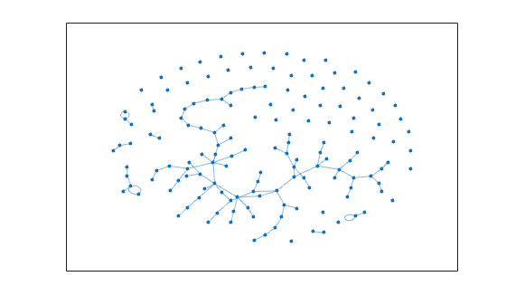
Update the layout coordinates of the graph object, and specify 'UseGravity' as true so that the components are laid out radially around the origin, with more space allotted for the larger components.
layout(h,'force','UseGravity',true)
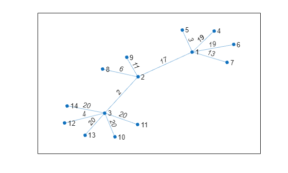
Graph Layout Based on Edge Weights
Plot a graph using the 'WeightEffect' name-value pair to make the length of graph edges proportional to their weights.
Create and plot a directed graph with weighted edges.
s = [1 1 1 1 1 2 2 2 3 3 3 3 3]; t = [2 4 5 6 7 3 8 9 10 11 12 13 14]; weights = randi([1 20],1,13); G = graph(s,t,weights); p = plot(G,'Layout','force','EdgeLabel',G.Edges.Weight);
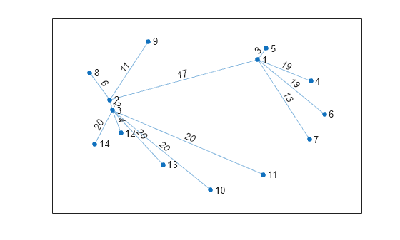
Recompute the layout of the graph using the 'WeightEffect' name-value pair, so that the length of each edge is proportional to its weight. This makes it so that the edges with the largest weights are the longest.
layout(p,'force','WeightEffect','direct')
Input Arguments
Input graph plot, specified as a GraphPlot object. Use the graph or digraph functions to create a graph, and then use plot with an output argument to return a GraphPlot object.
Example: H = plot(G)
method — Layout method
'auto' (default) | 'circle' | 'force' | 'layered' | 'subspace' | 'force3' | 'subspace3'
Layout method, specified as one of the options in the table. The table also lists compatible name-value pairs to further refine each layout method.
| Option | Description | Layout-Specific Name-Value Pairs |
|---|---|---|
| 'auto' (default) | Automatic choice of layout method based on the size and structure of the graph. | — |
| 'circle' | Circular layout. Places the graph nodes on a circle centered at the origin with radius 1. | 'Center' — Center node in circular layout |
| 'force' | Force-directed layout [1]. Uses attractive forces between adjacent nodes and repulsive forces between distant nodes. | 'Iterations' — Number of force-directed layout iterations'WeightEffect' — Effect of edge weights on layout'UseGravity' — Gravity toggle for layouts with multiple components'XStart' — Starting _x_-coordinates for nodes'YStart' — Starting_y_-coordinates for nodes |
| 'layered' | Layered layout [2], [3], [4]. Places the graph nodes into a set of layers, revealing hierarchical structure. By default the layers progress downwards (the arrows of a directed acyclic graph point down). | 'Direction' — Direction of layers'Sources' — Nodes to include in the first layer'Sinks' — Nodes to include in the last layer'AssignLayers' — Layer assignment method |
| 'subspace' | Subspace embedding layout [5]. Plots the graph nodes in a high-dimensional embedded subspace, and then projects the positions back into 2-D. By default the subspace dimension is either 100 or the total number of nodes, whichever is smaller. | 'Dimension' — Dimension of embedded subspace |
| 'force3' | 3-D force-directed layout. | 'Iterations' — Number of force-directed layout iterations'WeightEffect' — Effect of edge weights on layout'UseGravity' — Gravity toggle for layouts with multiple components'XStart' — Starting _x_-coordinates for nodes'YStart' — Starting_y_-coordinates for nodes'ZStart' — Starting _z_-coordinates for nodes |
| 'subspace3' | 3-D subspace embedding layout. | 'Dimension' — Dimension of embedded subspace |
Example: layout(H,'layered')
Example: layout(H,'force3','Iterations',10)
Example: layout(H,'subspace','Dimension',50)
Name-Value Arguments
Specify optional pairs of arguments asName1=Value1,...,NameN=ValueN, where Name is the argument name and Value is the corresponding value. Name-value arguments must appear after other arguments, but the order of the pairs does not matter.
Before R2021a, use commas to separate each name and value, and enclose Name in quotes.
Example: layout(H,'subspace','Dimension',200)
Force
Iterations — Number of force-directed layout iterations
100 (default) | positive scalar integer
Number of force-directed layout iterations, specified as the comma-separated pair consisting of 'Iterations' and a positive scalar integer.
This option is available only when method is'force' or 'force3'.
Example: layout(H,'force','Iterations',250)
Data Types: single | double | int8 | int16 | int32 | int64 | uint8 | uint16 | uint32 | uint64
WeightEffect — Effect of edge weights on layout
'none' (default) | 'direct' | 'inverse'
Effect of edge weights on layout, specified as the comma-separated pair consisting of 'WeightEffect' and one of the values in this table. If there are multiple edges between two nodes (as in a directed graph with an edge in each direction, or a multigraph), then the weights are summed before computing'WeightEffect'.
This option is available only when method is'force' or 'force3'.
| Value | Description |
|---|---|
| 'none' (default) | Edge weights do not affect the layout. |
| 'direct' | Edge length is proportional to the edge weight,G.Edges.Weight. Larger edge weights produce longer edges. |
| 'inverse' | Edge length is inversely proportional to the edge weight, 1./G.Edges.Weight. Larger edge weights produce shorter edges. |
Example: layout(H,'force','WeightEffect','inverse')
UseGravity — Gravity toggle for layouts with multiple components
'off' orfalse (default) | 'on' or true
Gravity toggle for layouts with multiple components, specified as the comma-separated pair consisting of 'UseGravity' and either 'off', 'on',true, or false. A value of'on' is equivalent to true, and 'off' is equivalent tofalse.
By default, MATLAB® lays out graphs with multiple components on a grid. The grid can obscure the details of larger components since they are given the same amount of space as smaller components. With'UseGravity' set to 'on' ortrue, multiple components are instead laid out radially around the origin. This layout spreads out the components in a more natural way, and provides more space for larger components.
This option is available only when method is'force' or 'force3'.
Example: layout(H,'force','UseGravity',true)
Data Types: char | logical
XStart — Starting x-coordinates for nodes
vector
Starting x-coordinates for nodes, specified as the comma-separated pair consisting of 'XStart' and a vector of node coordinates. Use this option together with 'YStart' to specify 2-D starting coordinates (or with 'YStart' and 'ZStart' to specify 3-D starting coordinates) before iterations of the force-directed algorithm change the node positions.
This option is available only when method is'force' or 'force3'.
Example: layout(H,'force','XStart',x,'YStart',y)
Data Types: single | double | int8 | int16 | int32 | int64 | uint8 | uint16 | uint32 | uint64
YStart — Starting y-coordinates for nodes
vector
Starting y-coordinates for nodes, specified as the comma-separated pair consisting of 'YStart' and a vector of node coordinates. Use this option together with 'XStart' to specify 2-D starting coordinates (or with 'XStart' and 'ZStart' to specify 3-D starting coordinates) before iterations of the force-directed algorithm change the node positions.
This option is available only when method is'force' or 'force3'.
Example: layout(H,'force','XStart',x,'YStart',y)
Example: layout(H,'force','XStart',x,'YStart',y,'ZStart',z)
Data Types: single | double | int8 | int16 | int32 | int64 | uint8 | uint16 | uint32 | uint64
ZStart — Starting z-coordinates for nodes
vector
Starting z-coordinates for nodes, specified as the comma-separated pair consisting of 'ZStart' and a vector of node coordinates. Use this option together with 'XStart' and 'YStart' to specify the starting_x_, y, and z node coordinates before iterations of the force-directed algorithm change the node positions.
This option is available only when method is'force3'.
Example: layout(H,'force','XStart',x,'YStart',y,'ZStart',z)
Data Types: single | double | int8 | int16 | int32 | int64 | uint8 | uint16 | uint32 | uint64
Layered
Direction — Direction of layers
'down' (default) | 'up' | 'left' | 'right'
Direction of layers, specified as the comma-separated pair consisting of 'Direction' and either 'down','up', 'left' or'right'. For directed acyclic (DAG) graphs, the arrows point in the indicated direction.
This option is available only when method is'layered'.
Example: layout(H,'layered','Direction','up')
Sources — Nodes to include in the first layer
node indices | node names
Nodes to include in the first layer, specified as the comma-separated pair consisting of 'Sources' and one or more node indices or node names.
This table shows the different ways to refer to one or more nodes either by their numeric node indices or by their node names.
| Form | Single Node | Multiple Nodes |
|---|---|---|
| Node index | ScalarExample: 1 | VectorExample: [1 2 3] |
| Node name | Character vectorExample: 'A' | Cell array of character vectorsExample: {'A' 'B' 'C'} |
| String scalarExample: "A" | String arrayExample: ["A" "B" "C"] |
This option is available only when method is'layered'.
Example: layout(H,'layered','Sources',[1 3 5])
Sinks — Nodes to include in the last layer
node indices | node names
Nodes to include in the last layer, specified as the comma-separated pair consisting of 'Sinks' and one or more node indices or node names.
This option is available only when method is'layered'.
Example: layout(H,'layered','Sinks',[2 4 6])
AssignLayers — Layer assignment method
'auto' (default) | 'asap' | 'alap'
Layer assignment method, specified as the comma-separated pair consisting of 'AssignLayers' and one of the options in this table.
| Option | Description |
|---|---|
| 'auto' (default) | Node assignment uses either 'asap' or 'alap', whichever is more compact. |
| 'asap' | As soon as possible. Each node is assigned to the first possible layer, given the constraint that all its predecessors must be in earlier layers. |
| 'alap' | As late as possible. Each node is assigned to the last possible layer, given the constraint that all its successors must be in later layers. |
This option is available only when method is'layered'.
Example: layout(H,'layered','AssignLayers','alap')
Subspace
Dimension — Dimension of embedded subspace
positive scalar integer
Dimension of embedded subspace, specified as the comma-separated pair consisting of 'Dimension' and a positive scalar integer.
- The default integer value is
min([100, numnodes(G)]). - For the
'subspace'layout, the integer must be greater than or equal to 2. - For the
'subspace3'layout, the integer must be greater than or equal to 3. - In both cases, the integer must be less than the number of nodes.
This option is available only when method is'subspace' or'subspace3'.
Example: layout(H,'subspace','Dimension',d)
Data Types: single | double | int8 | int16 | int32 | int64 | uint8 | uint16 | uint32 | uint64
Circle
Center — Center node in circular layout
node index | node name
Center node in circular layout, specified as the comma-separated pair consisting of 'Center' and one of the values in this table.
| Value | Example |
|---|---|
| Scalar node index | 1 |
| Character vector node name | 'A' |
| String scalar node name | "A" |
This option is available only when method is'circle'.
Example: layout(H,'circle','Center',3) places node three at the center.
Example: layout(H,'circle','Center','Node1') places the node named 'Node1' at the center.
Tips
- Use the
Layoutname-value pair to change the layout of a graph when you plot it. For example,plot(G,'Layout','circle')plots the graphGwith a circular layout. - When using the
'force'or'force3'layout methods, a best practice is to use more iterations with the algorithm instead of usingXStart,YStart, andZStartto restart the algorithm using previous outputs. The result of executing the algorithm with 100 iterations is different in comparison to executing 50 iterations, and then restarting the algorithm from the ending positions to execute 50 more iterations.
References
[1] Fruchterman, T., and E. Reingold,. “Graph Drawing by Force-directed Placement.” Software — Practice & Experience. Vol. 21 (11), 1991, pp. 1129–1164.
[2] Gansner, E., E. Koutsofios, S. North, and K.-P Vo. “A Technique for Drawing Directed Graphs.” IEEE Transactions on Software Engineering. Vol.19, 1993, pp. 214–230.
[3] Barth, W., M. Juenger, and P. Mutzel. “Simple and Efficient Bilayer Cross Counting.” Journal of Graph Algorithms and Applications. Vol.8 (2), 2004, pp. 179–194.
[4] Brandes, U., and B. Koepf. “Fast and Simple Horizontal Coordinate Assignment.” LNCS. Vol. 2265, 2002, pp. 31–44.
[5] Y. Koren. “Drawing Graphs by Eigenvectors: Theory and Practice.” Computers and Mathematics with Applications. Vol. 49, 2005, pp. 1867–1888.
Version History
Introduced in R2015b