Types of Autoencoders (original) (raw)

Last Updated : 9 Oct, 2025

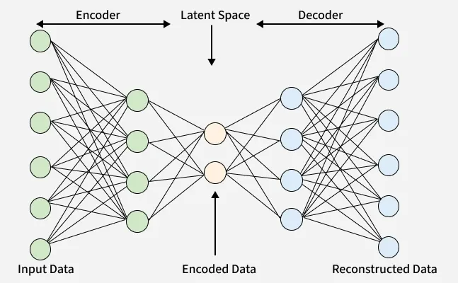
Autoencoders are a type of neural network designed to learn efficient data representations. They work by compressing input data into a smaller, dense format called the latent space using an encoder and then reconstructing the original input from this compressed form using a decoder. This makes autoencoders useful for tasks such as dimensionality reduction, feature extraction and noise removal.

Autoencoders

Let’s see common types of autoencoders which are designed with unique features to handle specific challenges and tasks in data representation and learning.

1. Vanilla Autoencoder

• Vanilla Autoencoder are the simplest form used for unsupervised learning tasks. They consist of two main parts an encoder that compresses the input data into a smaller, dense representation and a decoder that reconstructs the original input from this compressed form.
• Training minimizes reconstruction error which measures the difference between input and output. This optimization is done via backpropagation which helps in updating the network weights to improve reconstruction accuracy.
• They are foundational models helps in serving as building blocks for more complex variants.

**Applications

Some key applications include:

• **Data Compression: They learn a compact version of the input data making storage and transmission more efficient.
• **Feature Learning: It extract important patterns from data which is useful in image processing, natural language processing and sensor analysis.
• **Anomaly Detection: If the reconstructed output is different from the original input, it can show an anomaly or outlier which makes autoencoders useful for fraud detection and system monitoring.

**Now lets see the practical implementation.

Here we will be using Numpy, Matplotlib and Tensorflow libraries for its implementation and also we are using inbuilt dataset for this.

• ****(x_train, _), (x_test, _) = fashion_mnist.load_data()**: Loads Fashion MNIST dataset into training and testing sets, ignoring labels.
• **encoded = tf.keras.layers.Dense(encoding_dim, activation='relu')(input_img): Encodes input into 32-dimensional vector with ReLU activation.
• **decoded = tf.keras.layers.Dense(784, activation='sigmoid')(encoded): Decodes the compressed vector back to 784 dimensions with sigmoid activation.
• **autoencoder = tf.keras.Model(input_img, decoded): Creates the autoencoder model connecting input to output. Python `

import numpy as np import matplotlib.pyplot as plt import tensorflow as tf from tensorflow.keras.datasets import fashion_mnist

(x_train, _), (x_test, _) = fashion_mnist.load_data() x_train = x_train.astype('float32') / 255. x_test = x_test.astype('float32') / 255.

x_train_flat = x_train.reshape(len(x_train), 784) x_test_flat = x_test.reshape(len(x_test), 784)

n = 10 encoding_dim = 32 input_img = tf.keras.Input(shape=(784,)) encoded = tf.keras.layers.Dense(encoding_dim, activation='relu')(input_img) decoded = tf.keras.layers.Dense(784, activation='sigmoid')(encoded)

autoencoder = tf.keras.Model(input_img, decoded) autoencoder.compile(optimizer='adam', loss='binary_crossentropy')

autoencoder.fit(x_train_flat, x_train_flat, epochs=50, batch_size=256, shuffle=True, validation_data=(x_test_flat, x_test_flat))

decoded_imgs = autoencoder.predict(x_test_flat)

plt.figure(figsize=(20, 4)) for i in range(n): ax = plt.subplot(2, n, i + 1) plt.imshow(x_test_flat[i].reshape(28, 28), cmap='gray') ax.axis('off')

ax = plt.subplot(2, n, i + 1 + n)
plt.imshow(decoded_imgs[i].reshape(28, 28), cmap='gray')
ax.axis('off')

plt.show()

`

**Output:

Results

2. Sparse Autoencoder

• Sparse Autoencoder add sparsity constraints that encourage only a small subset of neurons in the hidden layer to activate at once helps in creating a more efficient and focused representation.
• Unlike vanilla models, they include regularization methods like L1 penalty and dropout to enforce sparsity.
• KL Divergence is used to maintain the sparsity level by matching the latent distribution to a predefined sparse target.
• This selective activation helps in feature selection and learning meaningful patterns while ignoring irrelevant noise.

Applications

• **Feature Selection: Highlights the most relevant features by encouraging sparse activation helps in improving interpretability.
• **Dimensionality Reduction: Creates efficient, low-dimensional representations by limiting active neurons.
• **Noise Reduction: Reduces irrelevant information and noise by activating only key neurons helps in improving model generalization.

**Now lets see the practical implementation.

• **encoded = tf.keras.layers.Dense(encoding_dim, activation='relu', activity_regularizer=tf.keras.regularizers.l1(1e-5))(input_img): Creates the encoded layer with ReLU activation and adds L1 regularization to encourage sparsity. Python `

import numpy as np import matplotlib.pyplot as plt import tensorflow as tf from tensorflow.keras.datasets import fashion_mnist

(x_train, _), (x_test, _) = fashion_mnist.load_data() x_train = x_train.astype('float32') / 255. x_test = x_test.astype('float32') / 255.

x_train_flat = x_train.reshape(len(x_train), 784) x_test_flat = x_test.reshape(len(x_test), 784)

n = 10 encoding_dim = 32 input_img = tf.keras.Input(shape=(784,)) encoded = tf.keras.layers.Dense(encoding_dim, activation='relu', activity_regularizer=tf.keras.regularizers.l1(1e-5))(input_img) decoded = tf.keras.layers.Dense(784, activation='sigmoid')(encoded)

sparse_autoencoder = tf.keras.Model(input_img, decoded) sparse_autoencoder.compile(optimizer='adam', loss='binary_crossentropy')

sparse_autoencoder.fit(x_train_flat, x_train_flat, epochs=50, batch_size=256, shuffle=True, validation_data=(x_test_flat, x_test_flat))

decoded_imgs = sparse_autoencoder.predict(x_test_flat)

plt.figure(figsize=(20, 4)) for i in range(n): ax = plt.subplot(2, n, i + 1) plt.imshow(x_test_flat[i].reshape(28, 28), cmap='gray') ax.axis('off')

ax = plt.subplot(2, n, i + 1 + n)
plt.imshow(decoded_imgs[i].reshape(28, 28), cmap='gray')
ax.axis('off')

plt.show()

`

**Output:

Results

3. Denoising Autoencoder

• **Denoising Autoencoders are designed to handle corrupted or noisy inputs by learning to reconstruct the clean, original data.
• Training involves feeding intentionally corrupted inputs and minimizing the reconstruction error against the clean version.
• This approach forces the model to capture robust features that are invariant to noise.

Applications

• **Image Denoising: Removes noise from images to increase quality and improve downstream processing.
• **Signal Cleaning: Filters noise from audio and sensor signals helps in boosting detection accuracy.
• **Data Preprocessing: Cleans corrupted data before input to other models helps in increasing robustness and performance.

**Now lets see the practical implementation.

Python `

import numpy as np import matplotlib.pyplot as plt import tensorflow as tf from tensorflow.keras.datasets import fashion_mnist

(x_train, _), (x_test, _) = fashion_mnist.load_data() x_train = x_train.astype('float32') / 255. x_test = x_test.astype('float32') / 255.

x_train_flat = x_train.reshape(len(x_train), 784) x_test_flat = x_test.reshape(len(x_test), 784)

n = 10 encoding_dim = 32 input_img = tf.keras.Input(shape=(784,)) encoded = tf.keras.layers.Dense(encoding_dim, activation='relu')(input_img) decoded = tf.keras.layers.Dense(784, activation='sigmoid')(encoded)

denoising_autoencoder = tf.keras.Model(input_img, decoded) denoising_autoencoder.compile(optimizer='adam', loss='binary_crossentropy')

noise_factor = 0.5 x_train_noisy = x_train_flat + noise_factor *
np.random.normal(loc=0.0, scale=1.0, size=x_train_flat.shape) x_test_noisy = x_test_flat + noise_factor *
np.random.normal(loc=0.0, scale=1.0, size=x_test_flat.shape) x_train_noisy = np.clip(x_train_noisy, 0., 1.) x_test_noisy = np.clip(x_test_noisy, 0., 1.)

denoising_autoencoder.fit(x_train_noisy, x_train_flat, epochs=50, batch_size=256, shuffle=True, validation_data=(x_test_noisy, x_test_flat))

decoded_imgs = denoising_autoencoder.predict(x_test_noisy)

plt.figure(figsize=(20, 6)) for i in range(n): ax = plt.subplot(3, n, i + 1) plt.imshow(x_test_flat[i].reshape(28, 28), cmap='gray') ax.axis('off')

ax = plt.subplot(3, n, i + 1 + n)
plt.imshow(x_test_noisy[i].reshape(28, 28), cmap='gray')
ax.axis('off')

ax = plt.subplot(3, n, i + 1 + 2 * n)
plt.imshow(decoded_imgs[i].reshape(28, 28), cmap='gray')
ax.axis('off')

plt.show()

`

**Output:

Results

4. Undercomplete Autoencoder

• **Undercomplete Autoencoders intentionally restrict the size of the hidden layer to be smaller than the input layer.
• This bottleneck forces the model to compress the data helps in learning only the most significant features and discarding redundant information.
• The model is trained by minimizing the reconstruction error while ensuring the latent space remains compact.

Applications

• **Anomaly Detection: Detects unusual data points by capturing deviations in compressed features.
• **Feature Extraction: Focuses on key data characteristics to improve classification and analysis.
• **Data Compression: Encodes input data efficiently to save storage and speed up transmission.

**Now lets see the practical implementation.

• **encoded = tf.keras.layers.Dense(encoding_dim, activation='relu',(input_img): Builds the encoder layer with ReLU activation. Python `

import numpy as np import matplotlib.pyplot as plt import tensorflow as tf from tensorflow.keras.datasets import fashion_mnist

(x_train, _), (x_test, _) = fashion_mnist.load_data() x_train = x_train.astype('float32') / 255. x_test = x_test.astype('float32') / 255.

x_train_flat = x_train.reshape(len(x_train), 784) x_test_flat = x_test.reshape(len(x_test), 784)

n = 10 encoding_dim = 16 input_img = tf.keras.Input(shape=(784,)) encoded = tf.keras.layers.Dense(encoding_dim, activation='relu')(input_img) decoded = tf.keras.layers.Dense(784, activation='sigmoid')(encoded)

undercomplete_autoencoder = tf.keras.Model(input_img, decoded) undercomplete_autoencoder.compile(optimizer='adam', loss='binary_crossentropy')

undercomplete_autoencoder.fit(x_train_flat, x_train_flat, epochs=50, batch_size=256, shuffle=True, validation_data=(x_test_flat, x_test_flat))

decoded_imgs = undercomplete_autoencoder.predict(x_test_flat)

plt.figure(figsize=(20, 4)) for i in range(n): ax = plt.subplot(2, n, i + 1) plt.imshow(x_test_flat[i].reshape(28, 28), cmap='gray') ax.axis('off')

ax = plt.subplot(2, n, i + 1 + n)
plt.imshow(decoded_imgs[i].reshape(28, 28), cmap='gray')
ax.axis('off')

plt.show()

`

**Output:

Results

5. Contractive Autoencoder

• **Contractive Autoencoders introduce an additional penalty during training to make the learned representations robust to small changes in input data.
• They minimize both reconstruction error and a regularization term that penalizes sensitivity to input perturbations.
• This results in stable, invariant features useful in noisy or fluctuating environments.

Applications

• **Stable Representation: Learns features that remain consistent despite small input variations.
• **Transfer Learning: Provides robust feature vectors for tasks with limited labeled data.
• **Data Augmentation: Generates stable variants of input data to increase training diversity.

**Now lets see the practical implementation.

Python `

import numpy as np import matplotlib.pyplot as plt import tensorflow as tf from tensorflow.keras.datasets import fashion_mnist

(x_train, _), (x_test, _) = fashion_mnist.load_data() x_train = x_train.astype('float32') / 255. x_test = x_test.astype('float32') / 255.

x_train_flat = x_train.reshape(len(x_train), 784) x_test_flat = x_test.reshape(len(x_test), 784)

n = 10 encoding_dim = 32 input_img = tf.keras.Input(shape=(784,)) encoded = tf.keras.layers.Dense(encoding_dim, activation='relu')(input_img) decoded = tf.keras.layers.Dense(784, activation='sigmoid')(encoded)

contractive_autoencoder = tf.keras.Model(input_img, decoded)

def contractive_loss(y_true, y_pred): mse = tf.keras.losses.mean_squared_error(y_true, y_pred) W = contractive_autoencoder.layers[1].kernel
dh = tf.gradients(contractive_autoencoder.layers[1].output, input_img)[0] contractive = tf.reduce_sum(tf.square(W)) * tf.reduce_sum(tf.square(dh)) return mse + 1e-4 * contractive

contractive_autoencoder.compile(optimizer='adam', loss='binary_crossentropy')

contractive_autoencoder.fit(x_train_flat, x_train_flat, epochs=50, batch_size=256, shuffle=True, validation_data=(x_test_flat, x_test_flat))

decoded_imgs = contractive_autoencoder.predict(x_test_flat)

plt.figure(figsize=(20, 4)) for i in range(n): ax = plt.subplot(2, n, i + 1) plt.imshow(x_test_flat[i].reshape(28, 28), cmap='gray') ax.axis('off')

ax = plt.subplot(2, n, i + 1 + n)
plt.imshow(decoded_imgs[i].reshape(28, 28), cmap='gray')
ax.axis('off')

plt.show()

`

**Output:

Results

6. Convolutional Autoencoder

• Convolutional Autoencoders use convolutional layers to effectively capture spatial and hierarchical features in high-dimensional data such as images.
• These models optimize reconstruction error using loss functions suited for images like mean squared error or binary cross-entropy.
• The architecture helps in handling structured inputs by preserving spatial relationships.

Applications

Convolutional autoencoders find applications in various domains where hierarchical features are important. Some applications include:

• **Image Reconstruction: Restores high-quality images from compressed latent codes.
• **Image Denoising: Removes noise while preserving spatial detail in images.
• **Feature Extraction: Captures hierarchical spatial features for tasks like classification and segmentation.

**Now lets see the practical implementation.

Python `

import numpy as np import matplotlib.pyplot as plt import tensorflow as tf from tensorflow.keras.datasets import fashion_mnist

(x_train, _), (x_test, _) = fashion_mnist.load_data() x_train = x_train.astype('float32') / 255. x_test = x_test.astype('float32') / 255.

x_train_flat = x_train.reshape(len(x_train), 784) x_test_flat = x_test.reshape(len(x_test), 784)

n = 10 input_img = tf.keras.Input(shape=(28, 28, 1))

x = tf.keras.layers.Conv2D( 16, (3, 3), activation='relu', padding='same')(input_img) x = tf.keras.layers.MaxPooling2D((2, 2), padding='same')(x) x = tf.keras.layers.Conv2D(8, (3, 3), activation='relu', padding='same')(x) encoded = tf.keras.layers.MaxPooling2D((2, 2), padding='same')(x)

x = tf.keras.layers.Conv2D( 8, (3, 3), activation='relu', padding='same')(encoded) x = tf.keras.layers.UpSampling2D((2, 2))(x) x = tf.keras.layers.Conv2D(16, (3, 3), activation='relu', padding='same')(x) x = tf.keras.layers.UpSampling2D((2, 2))(x) decoded = tf.keras.layers.Conv2D( 1, (3, 3), activation='sigmoid', padding='same')(x)

conv_autoencoder = tf.keras.Model(input_img, decoded) conv_autoencoder.compile(optimizer='adam', loss='binary_crossentropy')

x_train_cnn = x_train.reshape(-1, 28, 28, 1) x_test_cnn = x_test.reshape(-1, 28, 28, 1)

conv_autoencoder.fit(x_train_cnn, x_train_cnn, epochs=50, batch_size=256, shuffle=True, validation_data=(x_test_cnn, x_test_cnn))

decoded_imgs = conv_autoencoder.predict(x_test_cnn)

plt.figure(figsize=(20, 4)) for i in range(n): ax = plt.subplot(2, n, i + 1) plt.imshow(x_test_cnn[i].reshape(28, 28), cmap='gray') ax.axis('off')

ax = plt.subplot(2, n, i + 1 + n)
plt.imshow(decoded_imgs[i].reshape(28, 28), cmap='gray')
ax.axis('off')

plt.show()

`

**Output:

Results

7. Variational Autoencoder

Variational Autoencoder (VAEs) extend traditional autoencoders by learning probabilistic latent distributions instead of fixed representations. Training optimizes the Evidence Lower Bound (ELBO) which balances:

1. **Reconstruction loss to ensure accurate data reconstruction.
2. **KL Divergence to regularize the latent space towards a standard Gaussian helps in preventing overfitting and smooth latent structure.

By balancing these two terms VAEs can generate meaningful outputs while keeping the latent space structured.

Applications

Here are some common applications:

• **Image Generation: Creates new realistic images by sampling from learned latent distributions.
• **Anomaly Detection: Identifies anomalies by measuring how well input data is reconstructed.
• **Dimensionality Reduction: Produces low-dimensional latent spaces useful for visualization and clustering.

**Now lets see the practical implementation.

• **x_train = np.reshape(x_train, (len(x_train), 28, 28, 1)) : Reshapes training images to 28x28 with 1 channel for Conv2D input.
• **input_img = tf.keras.Input(shape=(28, 28, 1)) : Defines input layer for grayscale images with shape 28x28x1.
• **tf.keras.layers.MaxPooling2D((2, 2), padding='same')(x) : Reduces spatial dimensions by half using max pooling with same padding.
• **decoded = tf.keras.layers.Conv2D(1, (3, 3), activation='sigmoid', padding='same')(x) : Outputs reconstructed image with 1 channel and sigmoid activation for pixel values between 0 and 1. Python `

import numpy as np import matplotlib.pyplot as plt import tensorflow as tf from tensorflow.keras import backend as K from tensorflow.keras.datasets import fashion_mnist

(x_train, _), (x_test, _) = fashion_mnist.load_data() x_train = x_train.astype('float32') / 255. x_test = x_test.astype('float32') / 255. x_train_cnn = x_train.reshape(-1, 28, 28, 1) x_test_cnn = x_test.reshape(-1, 28, 28, 1)

latent_dim = 2 n = 10

encoder_inputs = tf.keras.Input(shape=(28, 28, 1)) x = tf.keras.layers.Conv2D(32, 3, activation='relu', strides=2, padding='same')(encoder_inputs) x = tf.keras.layers.Conv2D(64, 3, activation='relu', strides=2, padding='same')(x) x = tf.keras.layers.Flatten()(x) x = tf.keras.layers.Dense(16, activation='relu')(x) z_mean = tf.keras.layers.Dense(latent_dim)(x) z_log_var = tf.keras.layers.Dense(latent_dim)(x)

def sampling(args): z_mean, z_log_var = args batch = tf.shape(z_mean)[0] dim = tf.shape(z_mean)[1] epsilon = tf.random.normal(shape=(batch, dim)) return z_mean + tf.exp(0.5 * z_log_var) * epsilon

z = tf.keras.layers.Lambda(sampling)([z_mean, z_log_var])

encoder = tf.keras.Model( encoder_inputs, [z_mean, z_log_var, z], name='encoder')

latent_inputs = tf.keras.Input(shape=(latent_dim,)) x = tf.keras.layers.Dense(7 * 7 * 64, activation='relu')(latent_inputs) x = tf.keras.layers.Reshape((7, 7, 64))(x) x = tf.keras.layers.Conv2DTranspose( 64, 3, strides=2, padding='same', activation='relu')(x) x = tf.keras.layers.Conv2DTranspose( 32, 3, strides=2, padding='same', activation='relu')(x) decoder_outputs = tf.keras.layers.Conv2DTranspose( 1, 3, padding='same', activation='sigmoid')(x)

decoder = tf.keras.Model(latent_inputs, decoder_outputs, name='decoder')

outputs = decoder(z)

class VAELossLayer(tf.keras.layers.Layer): def init(self, **kwargs): super(VAELossLayer, self).init(**kwargs)

def call(self, inputs):
    x, x_decoded, z_mean, z_log_var = inputs

    reconstruction_loss = tf.keras.losses.binary_crossentropy(
        K.flatten(x), K.flatten(x_decoded)
    )
    reconstruction_loss *= 28 * 28

    kl_loss = 1 + z_log_var - K.square(z_mean) - K.exp(z_log_var)
    kl_loss = K.sum(kl_loss, axis=-1)
    kl_loss *= -0.5

    total_loss = K.mean(reconstruction_loss + kl_loss)
    self.add_loss(total_loss)
    return x_decoded

outputs_with_loss = VAELossLayer()( [encoder_inputs, outputs, z_mean, z_log_var])

vae = tf.keras.Model(encoder_inputs, outputs_with_loss, name='vae_with_loss')

vae.compile(optimizer='adam')

vae.fit(x_train_cnn, epochs=50, batch_size=256, validation_data=(x_test_cnn, None))

decoded_imgs = vae.predict(x_test_cnn)

plt.figure(figsize=(20, 4)) for i in range(n): ax = plt.subplot(2, n, i + 1) plt.imshow(x_test_cnn[i].reshape(28, 28), cmap='gray') ax.axis('off')

ax = plt.subplot(2, n, i + 1 + n)
plt.imshow(decoded_imgs[i].reshape(28, 28), cmap='gray')
ax.axis('off')

plt.show()

`

**Output:

Results

By choosing the right type of autoencoder, we can solve a range of problems effectively and make the most of our data.

You can download source code from here.