Introduction to Matrices (original) (raw)
Last Updated : 20 Mar, 2026
Matrices are rectangular arrays of numbers, symbols, or characters where all of these elements are arranged in each row and column.
- A matrix is identified by its order, which is given in the form of rows ⨯ columns, and the location of each element is given by the row and column it belongs to.
- A matrix is represented as ([P]m⨯n), where P is the matrix, m is the number of rows, and n is the number of columns.
Given below is a general example of a matrix:
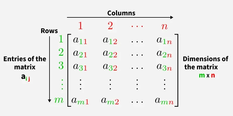
Figure 1: An (m ✖ n) Matrix
In mathematics, matrices are mainly used to represent and solve systems of linear equations, perform linear transformations, and study concepts like eigenvalues, determinants, and vector spaces.
Some common examples of matrices are
A =\begin{bmatrix} 1 & 2 \\ 3 &4 \\ \end{bmatrix}_{2\times 2} and B = \begin{bmatrix} 1 & -1 & 2 \\ 3 & 2 & 6 \\ 4 & -2& 5\\\end{bmatrix}_{3 \times3}
Here, A is a 2×2 matrix (2 rows and 2 columns) and B is a 3×3 matrix (3 rows and 3 columns).
Order of Matrix
The order of a matrix tells about the number of rows and columns present in a matrix. The order of a matrix is represented as the number of rows times the number of columns. Let's say if a matrix has 4 rows and 5 columns, then the order of the matrix will be 4⨯ 5. Always remember that the first number in the order signifies the number of rows present in the matrix, and the second number signifies the number of columns in the matrix.
Operations on Matrices
We can perform various mathematical operations on matrices, such as addition, subtraction, scalar multiplication, and multiplication. These operations are performed between the elements of two matrices to give an equivalent matrix that contains the elements that are obtained as a result of the operation between the elements of two matrices.
Addition of Matrices
In matrix addition or subtraction of matrices, the operation is performed between two matrices of the same order to yield a matrix that contains elements obtained by performing the operations on the elements of the two matrices.
The addition of matrices A and B:
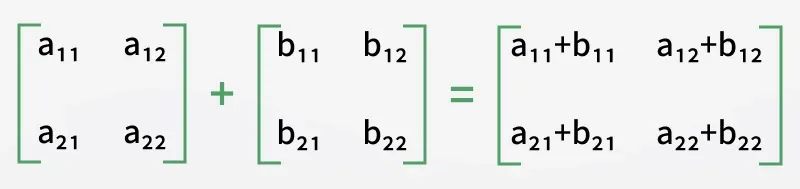
Figure 2: Adding two 2×2 matrices.
**Example: Find the sum of \bold{\begin{bmatrix} 1 & 2\\ 4& 5 \\ \end{bmatrix}}and \bold{\begin{bmatrix} 2 & 3 \\ 6 & 7 \\ \end{bmatrix}}
**Solution:
Here, we have A = \begin{bmatrix} 1 & 2\\ 4& 5 \\ \end{bmatrix}and B = \begin{bmatrix} 2 & 3 \\ 6 & 7 \\ \end{bmatrix}
A + B = \begin{bmatrix} 1& 2\\ 4& 5\\ \end{bmatrix}+ \begin{bmatrix} 2 & 3 \\ 6 & 7 \\ \end{bmatrix}
⇒ A + B = \begin{bmatrix} 1 + 2 & 2 + 3\\ 4 + 6& 5 + 7\\ \end{bmatrix}= \begin{bmatrix} 3 & 5\\ 10& 12\\ \end{bmatrix}
**Subtraction of Matrices
The subtraction of two matrices can be represented in terms of the addition of two matrices. Let's say we have to subtract matrix B from matrix A; then we can write A - B. We can also rewrite it as A + (-B).
The subtraction of matrices A and B:
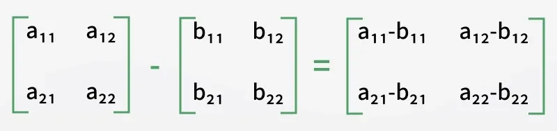
Figure 3: Subtracting two 2×2 matrices.
**Example: Subtract \bold{\begin{bmatrix} 1 & 2\\ 4& 5 \\ \end{bmatrix}}from \bold{\begin{bmatrix} 2 & 3 \\ 6 & 7 \\ \end{bmatrix} }.
**Solution:
Let us assume A = \begin{bmatrix} 2 & 3 \\ 6 & 7 \\ \end{bmatrix}and B = \begin{bmatrix} 1 & 2\\ 4& 5 \\ \end{bmatrix}
A - B = \begin{bmatrix} 2 & 3 \\ 6 & 7 \\ \end{bmatrix}- \begin{bmatrix} 1 & 2\\ 4& 5 \\ \end{bmatrix}
⇒ A - B = \begin{bmatrix} 2 - 1 & 3 - 2 \\ 6 - 4 & 7 - 5 \\ \end{bmatrix}= \begin{bmatrix} 1 & 1 \\ 2 & 2 \\ \end{bmatrix}
Scalar Multiplication of Matrices
Scalar multiplication of matrices refers to the multiplication of each term of a matrix by a scalar. If a scalar, let's say 'k,' is multiplied by a matrix, then the equivalent matrix will contain elements equal to the product of the scalar and the element of the original matrix. Let's see an example:

Figure 4: Multiplying a matrix by a scalar (k)
**Example: Multiply 3 \bold{\begin{bmatrix} 1 & 2\\ 4& 5 \\ \end{bmatrix}}.
**Solution:
3[A] = \begin{bmatrix} 3\times1 & 3\times 2\\ 3\times4& 3\times5 \\ \end{bmatrix}
⇒ 3[A] = \begin{bmatrix} 3 & 6\\ 12& 15 \\ \end{bmatrix}
Multiplication of Matrices
In the multiplication of matrices, two matrices are multiplied to yield a single equivalent matrix. The multiplication is performed in the manner that the elements of the row of the first matrix multiply with the elements of the columns of the second matrix, and the product of the elements is added to yield a single element of the equivalent matrix. If a matrix [A]i⨯j is multiplied by matrix [B]j⨯k, then the product is given as [AB]i⨯k.
Matrix multiplication between matrices A and B is possible only if the number of columns of A is equal to the number of rows of B.
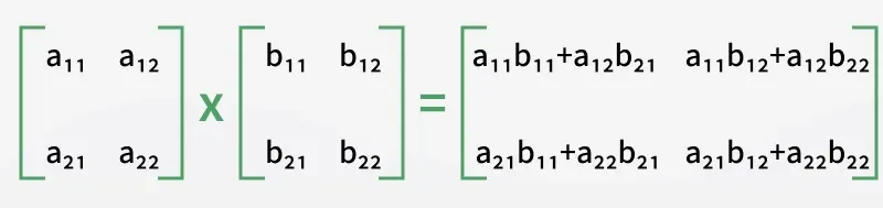
Figure 5: Product of two 2×2 matrices
**Example: Find the product of \bold{\begin{bmatrix} 1 & 2\\ 4& 5 \\ \end{bmatrix}}and \bold{\begin{bmatrix} 2 & 3 \\ 6 & 7 \\ \end{bmatrix}}
**Solution:
Let A = \begin{bmatrix} 1 & 2\\ 4& 5 \\ \end{bmatrix}and B = \begin{bmatrix} 2 & 3 \\ 6 & 7 \\ \end{bmatrix}
⇒ AB = \begin{bmatrix} 1 & 2\\ 4& 5 \\ \end{bmatrix}\begin{bmatrix} 2 & 3 \\ 6 & 7 \\ \end{bmatrix}
⇒ AB = \begin{bmatrix} 1\times2+2\times6 & 1\times3+2\times7\\ 4\times2+5\times6& 4\times3+5\times7 \\ \end{bmatrix}
⇒ AB = \begin{bmatrix} 14 & 17\\ 38& 47 \\ \end{bmatrix}
Transpose
The transpose of a matrix is the rearrangement of row elements in columns and column elements in a row to yield an equivalent matrix. A matrix in which the elements of the row of the original matrix are arranged in columns or vice versa is called a transpose matrix. The transpose matrix is represented as AT. If A = [aij]mxn, then AT = [bij]nxm, where bij = aji.
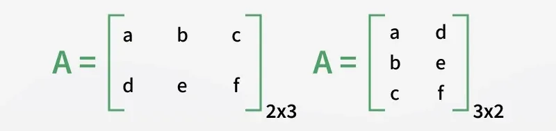
Figure 6: Transposing a 2×3 matrix to a 3×2 matrix.
**Example: Transpose of \begin{bmatrix} 18 & 17\\ 38& 47 \\ \end{bmatrix} ****.**
**Solution:
Let A = \begin{bmatrix} 18 & 17\\ 38& 47 \\ \end{bmatrix}
⇒ AT = \begin{bmatrix} 18 & 38\\ 17& 47 \\ \end{bmatrix}
Trace
The trace of a matrix is the sum of the principal diagonal elements of a square matrix. The trace of a matrix is only found in the case of a square matrix because diagonal elements exist only in square matrices. Let's see an example.
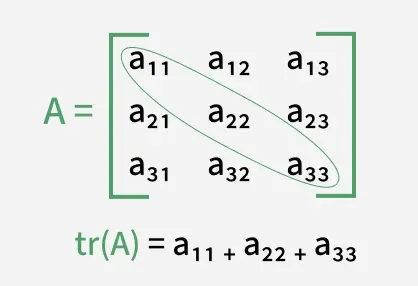
Figure 7: Trace of a 3×3 matrix
**Example: Find the trace of the matrix\begin{bmatrix} 1 & 2 & 3\\ 4 & 5 & 6\\ 7 & 8 & 9 \end{bmatrix}
**Solution:
Let us assume A = \begin{bmatrix} 1 & 2 & 3\\ 4 & 5 & 6\\ 7 & 8 & 9 \end{bmatrix}
Trace(A) = 1 + 5 + 9 = 15
Types of Matrices
Based on the number of rows and columns present and the special characteristics shown, types of matrices are classified into various types.
- **Row Matrix: A matrix that has only one row and one or more columns is called a row matrix.
- **Column Matrix****:** A matrix that has only one column and one or more rows is called a column matrix.
- **Horizontal Matrix: A matrix in which the number of rows is less than the number of columns is called a horizontal matrix.
- **Vertical Matrix: A matrix in which the number of columns is less than the number of rows is called a vertical matrix.
- **Rectangular Matrix****:** A matrix in which the number of rows and columns is unequal is called a rectangular matrix.
- **Square Matrix****:** A matrix in which the number of rows and columns is the same is called a square matrix.
- **Diagonal Matrix****:** A square matrix in which the non-diagonal elements are zero is called a diagonal matrix.
- **Zero or Null Matrix****:** A matrix whose all elements are zero is called a zero matrix. A zero matrix is also called a null matrix.
- **Unit or Identity Matrix****:** A diagonal matrix whose diagonal elements are all 1 is called a unit matrix. A unit matrix is also called an identity matrix. An identity matrix is represented by I.
- **Symmetric matrix****:** A square matrix is said to be symmetric if the transpose of the original matrix is equal to its original matrix. i.e., (AT) = A.
- **Skew-symmetric Matrix****:** A skew-symmetric (or antisymmetric or antimetric [1]) matrix is a square matrix whose transpose equals its negative, i.e., (AT) = -A.
- **Orthogonal Matrix****:** A matrix is said to be orthogonal if AAT = ATA = I
- **Idempotent Matrix: A matrix is said to be idempotent if A2 = A
- **Involutory Matrix: A matrix is said to be involutory if A2 = I.
- **Upper Triangular Matrix****:** A square matrix in which all the elements below the diagonal are zero is known as the upper triangular matrix
- **Lower Triangular Matrix****:** A square matrix in which all the elements above the diagonal are zero is known as the lower triangular matrix
- **Singular Matrix****:** A square matrix is said to be a singular matrix if its determinant is zero, i.e., |A|=0
- **Non-singular Matrix****:** A square matrix is said to be a non-singular matrix if its determinant is non-zero.
**Note: Every Square Matrix can uniquely be expressed as the sum of a symmetric matrix and a skew-symmetric matrix. A = 1/2 (AT + A) + 1/2 (A - AT).
Determinant of a Matrix
The determinant of a matrix is a numerical value associated with a square matrix. It is defined only for square matrices and is denoted by ∣A∣. The determinant is calculated using cofactor expansion, which involves multiplying each element of a row (or column) by its corresponding cofactor and then adding the results.
v
**Example 1: How to find the determinant of a 2⨯2 square matrix?
**Solution:
Let say we have matrix A = \begin{bmatrix} a & b \\ c & d \end{bmatrix}
Then, determinant is of A is |A| = ad - bc
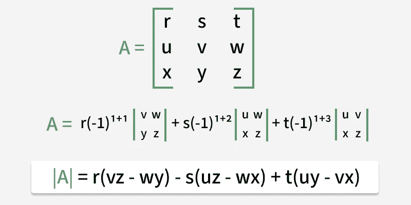
**Example 2: How to find the determinant of a 3⨯3 square matrix?
**Solution:
Let's say we have a 3⨯3 matrix A = \begin{bmatrix} a & b& c \\ d & e & f \\ g & h &i \\ \end{bmatrix}
Then |A| = a(-1)1+1\begin{vmatrix} e& f \\ h & i\\ \end{vmatrix}+ b(-1)1+2\begin{vmatrix} d& f \\ g & i\\ \end{vmatrix} + c(-1)1+3\begin{vmatrix} d& e \\ g & h\\ \end{vmatrix}
Minor of a Matrix
The minor of a matrix for an element is given by the determinant of a matrix obtained after deleting the row and column to which the particular element belongs. A minor of a matrix is represented by Mij. Let's see an example.
**Example: Find the minor of the matrix \begin{bmatrix} a & b& c \\ d & e & f \\ g & h &i \\ \end{bmatrix}for the element 'a.'
**Solution:
Minor of element 'a' is given as M11 = \begin{vmatrix} e& f \\ h & i\\ \end{vmatrix}
Cofactor of a Matrix
The cofactor of a matrix is found by multiplying the minor of the matrix for a given element by (-1)i+j. The cofactor of a matrix is represented as Cij. Hence, the relation between the minor and cofactor of a matrix is given as Cij = (-1)i+jMij. If we arrange all the cofactors obtained for an element, t, then we get a cofactor matrix given as C = \begin{bmatrix} c_{11} & c_{12}& c_{13} \\ c_{21} & c_{22} & c_{23} \\ c_{31} & c_{32} &c_{33} \\ \end{bmatrix}
Adjoint of a Matrix
The adjoint is calculated for a square matrix. The adjoint of a matrix is the transpose of the cofactor of the matrix. The adjoint of a matrix is thus expressed as adj(A) = CT, where C is the cofactor matrix.
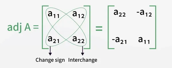
Figure 7: Adjoint of a 2×2 matrix
Let's say, for example, we have a matrix:
A = \begin{bmatrix} a_1 & b_1 & c_1\\ a_2 & b_2 & c_2\\ a_3 & b_3 & c_3 \end{bmatrix}
then:
\mathrm{adj(A)} = \begin{bmatrix} A_1 & B_1 & C_1\\ A_2 & B_2 & C_2\\ A_3 & B_3 & C_3 \end{bmatrix}^T \\ \Rightarrow \mathrm{adj(A)} =\begin{bmatrix} A_1 & A_2 & A_3\\ B_1 & B_2 & B_3\\ C_1 & C_2 & C_3 \end{bmatrix}
where,
\begin{bmatrix} A_1 & B_1 & C_1\\ A_2 & B_2 & C_2\\ A_3 & B_3 & C_3 \end{bmatrix}is a cofactor of Matrix A.
**Inverse of a Matrix
For a square matrix A of order n, its inverse A⁻¹ can be defined as a matrix that, when multiplied by the original matrix, generates an identity matrix I of order n. i.e., A×A⁻¹= I. The inverse is only calculated for a square matrix whose determinant is non-zero.
The formula for the inverse of a matrix is given as:
A-1 = adj(A)/det(A) = (1/|A|)(Adj A),
where |A| should not be equal to zero, which means matrix A should be non-singular.
Elementary Operations on Matrices
Elementary operations on matrices are performed to solve the linear equation and to find the inverse of a matrix. Elementary operations are between rows and between columns. There are three types of elementary operations performed for rows and columns. These operations are mentioned below:
Elementary operations include:
- Interchanging two rows/columns
- Multiplying a row/column by a non-zero number
- Adding two rows/columns
Rank of a Matrix
The rank of a matrix is given by the maximum number of linearly independent rows or columns of a matrix. The rank of a matrix is always less than or equal to the total number of rows or columns present in a matrix. A square matrix has linearly independent rows or columns if the matrix is non-singular, i.e., the determinant is not equal to zero. Since a zero matrix has no linearly independent rows or columns, its rank is zero. The rank of the matrix A is represented by ρ(A).
Matrix Formulas
- A-1 = adj(A)/| A|
- A(adj A) = (adj A)A = |A|I, where I is an Identity Matrix
- |adj A| = |A|n-1 where n is the order of matrix A
- adj(adj A) = |A|n-2A where n is the order of the matrix
- |adj(adj A)| = |A|(n-1)^2
- adj(AB) = (adj B)(adj A)
- adj(Ap) = (adj A)p
- adj(kA) = kn-1(adj A), where k is any real number
- adj(I) = I
- adj 0 = 0
- If A is symmetric, then adj(A) is also symmetric
- If A is a diagonal Matrix, then adj(A) is also a diagonal matrix
- If A is a triangular matrix, then adj(A) is also a triangular matrix
- If A is a singular matrix, then |adj A| = 0
- (AB)-1 = B-1A-1
Why Matrices Matter in Data Science
- **Efficient Data Representation: Tabular data (like datasets in CSV files or spreadsheets) can be easily stored as matrices.
- **Foundation for ML Models: Algorithms like linear regression, neural networks, and PCA use matrix operations.
- **Vectorized Computation: Libraries like NumPy, TensorFlow, and PyTorch use matrix operations to speed up calculations using hardware acceleration (CPU/GPU).
- **Multivariate Data: Datasets with multiple features per observation are naturally represented as matrices.
Common Uses of Matrices in Data Science
**1. Storing Datasets: Each row is an observation (e.g., a customer), and each column is a feature (e.g., age, income). For example:
**2. Linear Algebra in Machine Learning:
Matrices are used for:
- Matrix multiplication in linear regression
- Gradient calculation in optimization
- Transformation and projection in dimensionality reduction (e.g., PCA)
**3. Image Processing: Images are represented as matrices (grayscale) or tensors (color images with RGB channels), where each pixel is a value in the matrix.
**4. Natural Language Processing (NLP): Matrices represent word embeddings or sentence vectors. For example, a word2vec model converts words into dense vectors and arranges them into a matrix.
**5. Recommender Systems: A user-item matrix stores preferences, which can be used for collaborative filtering using matrix factorization.
Practice Problems Based on Introduction to Matrices
**Question 1. Find the sum of the matrices A = \begin{bmatrix} 3 & 4 \\ 7 & 8 \end{bmatrix} and \quad B = \begin{bmatrix} 1 & 2 \\ 5 & 6 \end{bmatrix}
**Question 2. Find the determinant of the matrix A = \begin{bmatrix} 4 & 3 \\ 2 & 1 \end{bmatrix}
**Question 3. Find the trace of the matrixA = \begin{bmatrix} 2 & 4 & 6 \\ 1 & 3 & 5 \\ 7 & 8 & 9 \end{bmatrix}
**Question 4. Find the product of the matrices A = \begin{bmatrix} 1 & 2 \\ 4 & 5 \end{bmatrix} and \quad B = \begin{bmatrix} 2 & 3 \\ 6 & 7 \end{bmatrix}
**Question 5. Find the inverse of the matrix (if possible). A = \begin{bmatrix} 1 & 2 \\ 3 & 4 \end{bmatrix}