Probability Distributions in R (original) (raw)

Last Updated : 29 Apr, 2026

In R, probability distributions (PD) describe the likelihood of different outcomes for a random variable. R provides functions for calculating, simulating and visualizing both continuous and discrete distributions, such as normal, binomial and Poisson. These functions include tools for probability mass functions (PMF), probability density functions (PDF), cumulative distribution functions (CDF) and random number generation.

Discrete Probability Distributions

Discrete probability distributions describe scenarios where the outcomes are distinct and countable. In R, these distributions allow for the modeling of various real-world situations. Below are the key types and their corresponding functions in R:

1. Binomial Distribution

The binomial distribution models the number of successes in a fixed number of independent Bernoulli trials.

**Functions:

• **dbinom(): Probability mass function
• **pbinom(): Cumulative distribution function
• **qbinom(): Quantile function
• **rbinom(): Random number generation

**Example: We want to simulate 100 random values based on a binomial distribution where each trial has 10 attempts (size = 10) with a probability of success (prob) of 0.5 in each trial. This means we are conducting 100 experiments where each experiment consists of 10 trials and each trial has a 50% chance of success.

R `

random_binom <- rbinom(10, size = 10, prob = 0.5) print(random_binom)

`

**Output:

Output

**Explanation:

• Since the Bernoulli distribution is just a binomial distribution with a single trial, we use rbinom() with size = 1 to generate values.
• The first argument (100) specifies that we want 100 random samples.
• The second argument (size = 1) specifies that each experiment has only one trial.
• The third argument (prob = 0.7) specifies the probability of success in each trial.
• Each output value is either 0 or 1, representing a failure or success in a single trial with a 70% chance of success.

2. Bernoulli Distribution

Bernoulli Distribution is a special case of the binomial distribution where the number of trials (size) is 1.

**Functions:

• **dbinom(): Probability mass function
• **pbinom(): Cumulative distribution function
• **qbinom(): Quantile function
• **rbinom(): Random number generation

These functions apply to the Bernoulli distribution by setting size = 1.

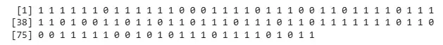
**Example: We want to simulate 100 random values based on a Bernoulli distribution, which is a special case of the binomial distribution where only 1 trial is conducted. Each trial has a probability of success of 0.7.

R `

random_bern <- rbinom(100, size = 1, prob = 0.7) print(random_bern)

`

**Output:

Output

**Explanation:

• Since the Bernoulli distribution is just a binomial distribution with a single trial, we use rbinom() with size = 1 to generate values.
• The first argument (100) specifies that we want 100 random samples.
• The second argument (size = 1) specifies that each experiment has only one trial.
• The third argument (prob = 0.7) specifies the probability of success in each trial.

3. Poisson Distribution

Poisson Distribution is used to model the number of events occurring within a fixed interval of time or space.

**Functions:

• **dpois(): Probability mass function.
• **ppois(): Cumulative distribution function.
• **qpois(): Quantile function.
• **rpois(): Random number generation.

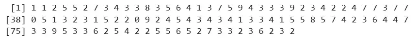
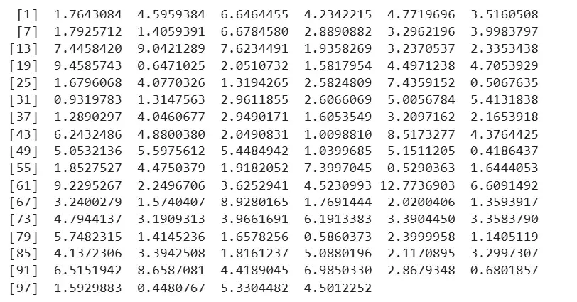
**Example: We want to simulate 100 random values based on a Poisson distribution. The Poisson distribution models the number of events happening in a fixed interval of time, where the average rate of occurrence is 4 events per interval (lambda = 4).

R `

random_pois <- rpois(100, lambda = 4) print(random_pois)

`

**Output:

Output

**Explanation:

• This function generates random values from a Poisson distribution.
• The first argument (100) specifies the number of random values we want to generate.
• The second argument (lambda = 4) specifies the average rate of occurrence of events (4 events per interval).
• Each output value represents the number of events that occur in a given interval, where the average number of events per interval is 4.

4. Geometric Distribution

Geometric Distribution is used to models the number of trials until the first success in a series of Bernoulli trials.

**Functions:

• **dgeom(): Probability mass function.
• **pgeom(): Cumulative distribution function.
• **qgeom(): Quantile function.
• **rgeom(): Random number generation.

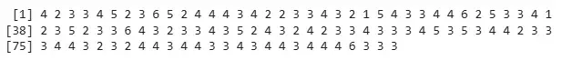
**Example: We want to simulate 100 random values based on a geometric distribution, which models the number of trials needed to get the first success in a series of Bernoulli trials, with a 30% chance of success per trial.

R `

random_geom <- rgeom(100, prob = 0.3) print(random_geom)

`

**Output:

Output

**Explanation:

• This function generates random values from a geometric distribution.
• The first argument (100) specifies that we want 100 random values.
• The second argument (prob = 0.3) specifies the probability of success on each trial (30%).
• Each output value represents the number of trials needed before the first success occurs in each experiment.

5. Hypergeometric Distribution

The hypergeometric distribution models the probability of k successes in n draws without replacement from a finite population containing a specific number of successes.

**Functions:

• **dhyper(): Probability mass function.
• **phyper(): Cumulative distribution function.
• **qhyper(): Quantile function.
• **rhyper(): Random number generation.

**Example: Draw 10 balls from a box of 20 total balls (7 red, 13 blue) and get red balls.

R `

random_hyper <- rhyper(100, m = 7, n = 13, k = 10) print(random_hyper)

`

**Output:

**Explanation:

Each number in the output is a possible outcome of red balls drawn in one random sample of size 10. For example:

• 4: means 4 red balls were drawn in that sample
• 2: 2 red balls drawn in that sample
• And so on, for 100 samples

The results vary between 1 and 6 red balls, which makes sense:

• Minimum red balls possible in 10 draws: max(0, 10 - 13) = 0, but here it starts from 1 due to randomness.
• Maximum red balls possible: min(10, 7) = 7, but the highest observed here is 6.

6. Multinomial Distribution in R

The multinomial distribution generalizes the binomial distribution for experiments with more than two possible outcomes.

**Functions:

• **rmultinom(): Random number generation

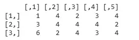
**Example: Toss a 3-sided die 10 times in 5 experiments.

R `

random_multinom <- rmultinom(5, size = 10, prob = c(0.2, 0.3, 0.5)) print(random_multinom)

`

**Output:

Output

**Explanation:

• Each column = one experiment (5 total).
• Each row = count of each die side (3 sides).
• Values show how often each side appeared in 10 tosses.
• Column totals = 10 (since each experiment has 10 tosses).

7. Negative Binomial Distribution

The negative binomial distribution models the number of failures before a set number of successes occurs.

**Functions:

• **dnbinom(): Probability mass function.
• **pnbinom(): Cumulative distribution function.
• **qnbinom(): Quantile function.
• **rnbinom(): Random number generation.

**Example: Simulate 100 values with 10 successes and 0.5 probability.

R `

random_nbinom <- rnbinom(100, size = 10, prob = 0.5) print(random_nbinom)

`

Explanation:

• 100 random values are generated from a negative binomial distribution.
• Each value shows failures before getting 10 successes with 0.5 success probability.
• Values vary based on how many failures occurred before 10 successes.

8. Benford’s Distribution

Benford's distribution or the first-digit law, predicts the distribution of the first digits in many real-life sets of numerical data. It is useful in fraud detection and data integrity checks.

**Functions:

**dbenford(): Probability mass function.
**pbenford(): Cumulative distribution function.
**rbenford(): Random number generation.

Continuous Probability Distributions

Continuous probability distributions model scenarios where the possible outcomes can take any value within a specified range. Instead of assigning probabilities to individual outcomes, these distributions provide probabilities for ranges of values.

1. Normal Distribution

The normal distribution is used to model continuous data that clusters around a mean, with data points symmetrically distributed around it.

**Functions:

• **dnorm(): Probability density function.
• **pnorm(): Cumulative distribution function.
• **qnorm(): Quantile function.
• **rnorm(): Random number generation.

**Example: We want to simulate 100 random values from a normal distribution with a mean of 0 and a standard deviation of 1. This is often used to model real-world data that tends to cluster around a central value (mean) with symmetric variation.

R `

random_norm <- rnorm(100, mean = 0, sd = 1) print(random_norm)

`

**Output:

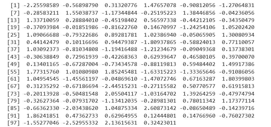
Output

**Explanation:

• This function generates random values from a normal distribution.
• The first argument (100) specifies the number of random values to generate.
• The second argument (mean = 0) specifies the mean of the distribution (the central value).
• The third argument (sd = 1) specifies the standard deviation (the spread or variability of the data).

By using this function, we generate 100 random values that follow a normal distribution with a mean of 0 and a standard deviation of 1.

2. Uniform Distribution

The uniform distribution models situations where all outcomes in a specified range have an equal chance of occurring.

**Functions:

• **dunif(): Probability density function.
• **punif(): Cumulative distribution function.
• **qunif(): Quantile function.
• **runif(): Random number generation.

**Example: We want to simulate 100 random values from a uniform distribution between 0 and 10, meaning each value within this range has an equal chance of occurring.

R `

random_unif <- runif(100, min = 0, max = 10) print(random_unif)

`

**Output:

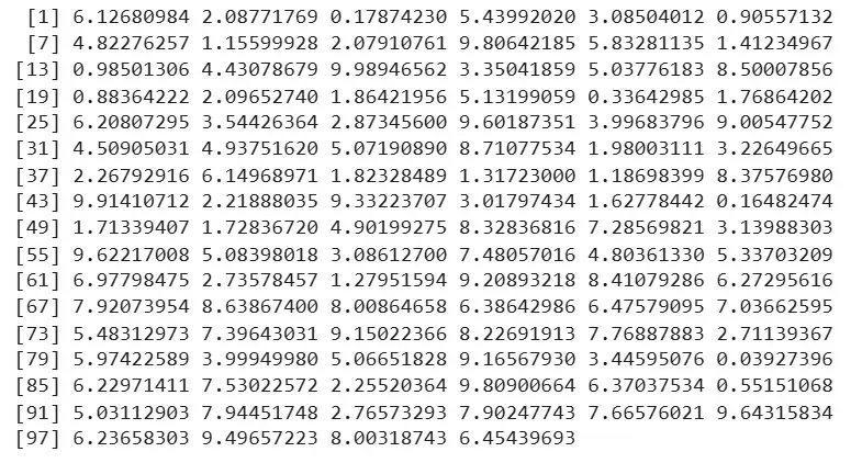
Output

**Explanation:

• runif() function generates random values from a uniform distribution.
• The first argument (100) specifies the number of random values to generate.
• The second argument (min = 0) specifies the minimum possible value.
• The third argument (max = 10) specifies the maximum possible value.
• Each value is equally likely to fall between 0 and 10.

3. Exponential Distribution

The exponential distribution is commonly used to model the time between events in a Poisson process, where events happen continuously and independently at a constant average rate.

**Functions:

• **dexp(): Probability density function.
• **pexp(): Cumulative distribution function.
• **qexp(): Quantile function.
• **rexp(): Random number generation.

**Example: We want to simulate 100 random values from an exponential distribution with a rate parameter of 0.2. This distribution is useful for modeling the time between events in a process where events occur continuously at a constant average rate.

R `

random_exp <- rexp(100, rate = 0.2) print(random_exp)

`

**Explanation:

• rexp() function generates random values from an exponential distribution.
• The first argument (100) specifies the number of random values to generate.
• The second argument (rate = 0.2) specifies the rate parameter, which controls the average time between events. A rate of 0.2 means the average time between events is 5 units.

By using this function, we generate 100 random values that represent the time between events in a Poisson process with a rate of 0.2.

4. Chi-Square Distribution

The Chi-Square distribution is used in hypothesis testing, especially for goodness-of-fit tests and in constructing confidence intervals for variance in normal distributions. It models the sum of squared standard normal variables.

**Functions:

• **dchisq(): Probability density function.
• **pchisq(): Cumulative distribution function.
• **qchisq(): Quantile function.
• **rchisq(): Random number generation.

**Example: The Chi-Square distribution is commonly used in Chi-Square tests to test the independence of categorical variables or in variance testing.

R `

random_chisq <- rchisq(100, df = 5) print(random_chisq)

`

**Output:

Output

**Explanation:

• rchisq() function generates random values from a Chi-Square distribution.
• The first argument (100) specifies how many random values we want to generate.
• The second argument (df = 5) specifies the degrees of freedom for the distribution, which is typically related to the number of variables or sample size.

5. Student's t-Distribution

The t-distribution is used when estimating population parameters with small sample sizes and unknown population variance. It has thicker tails than the normal distribution.

**Functions:

• **dt(): Probability density function.
• **pt(): Cumulative distribution function.
• **qt(): Quantile function.
• **rt(): Random number generation.

**Example: The t-distribution is widely used in t-tests for small sample sizes and for constructing confidence intervals for the population mean when the population variance is unknown.

R `

random_t <- rt(100, df = 10) print(random_t)

`

**Output:

Output

**Explanation:

• rt() function generates random values from a Student's t-distribution.
• The first argument (100) specifies the number of random values to generate.
• The second argument (df = 10) specifies the degrees of freedom, typically related to the sample size (usually n - 1 where n is the sample size).

6. Gamma Distribution

The Gamma distribution models the time until a certain number of events occur in a Poisson process. It is used in reliability analysis and queuing theory.

**Functions:

• **dgamma(): Probability density function.
• **pgamma(): Cumulative distribution function.
• **qgamma(): Quantile function.
• **rgamma(): Random number generation.

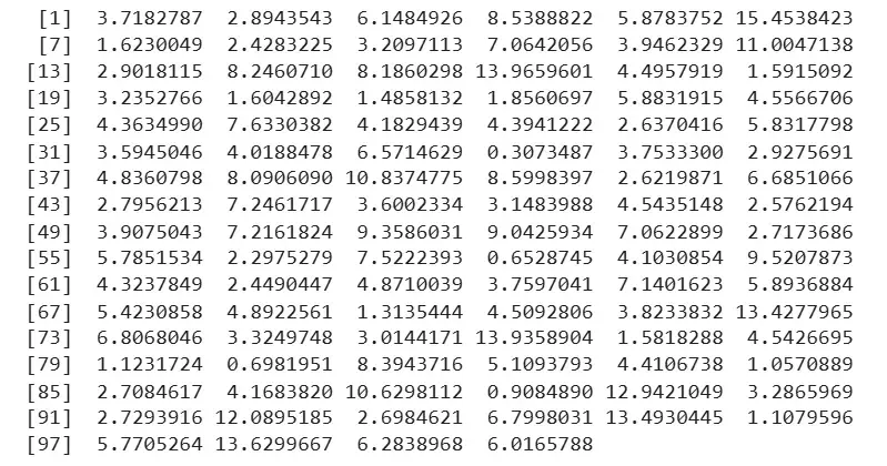
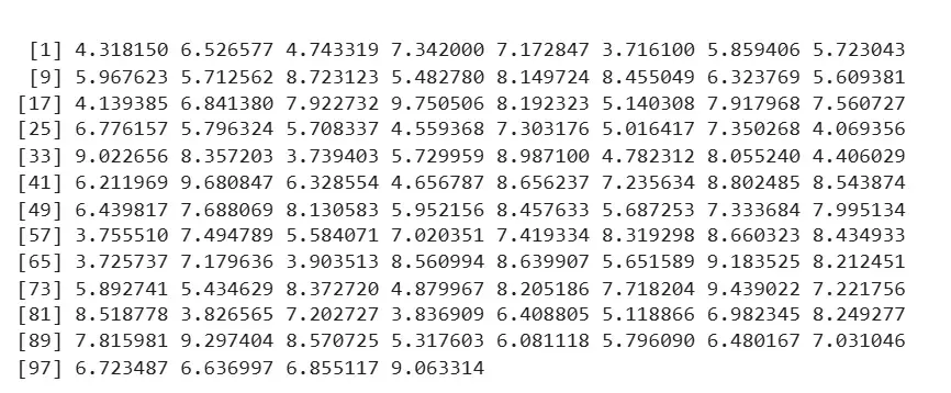
**Example: The Gamma distribution is frequently used in reliability analysis (e.g., modeling the time until a machine failure) and queuing theory (e.g., modeling the time between customer arrivals).

R `

random_gamma <- rgamma(100, shape = 2, rate = 0.5) print(random_gamma)

`

**Output:

Output

**Explanation:

• rgamma() function generates random values from a Gamma distribution.
• The first argument (100) specifies the number of random values to generate.
• The second argument (shape = 2) specifies the shape parameter, which affects the distribution's skewness.
• The third argument (rate = 0.5) specifies the rate parameter, which controls how quickly events occur (a higher rate results in more frequent events).

7. Beta Distribution

The Beta distribution models probabilities and proportions, commonly used in Bayesian statistics for prior distributions.

**Functions:

• **dbeta(): Probability density function
• **pbeta(): Cumulative distribution function
• **qbeta(): Quantile function
• **rbeta(): Random number generation

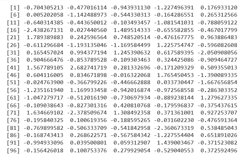
**Example: The Beta distribution is frequently used in Bayesian statistics to model the prior distribution of probabilities and in risk analysis to model uncertain probabilities of success.

R `

random_beta <- rbeta(100, shape1 = 2, shape2 = 5) print(random_beta)

`

**Output:

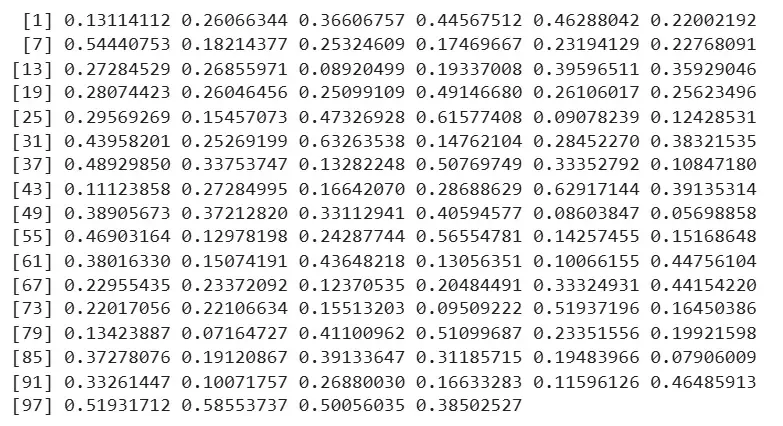
Output

**Explanation:

• rbeta() function generates random values from a Beta distribution.
• The first argument (100) specifies how many random values to generate.
• The second argument (shape1 = 2) specifies the first shape parameter (affecting the distribution's skewness).
• The third argument (shape2 = 5) specifies the second shape parameter.

8. Triangular Distribution

The triangular distribution is a continuous probability distribution with a shape that resembles a triangle. It is defined by three parameters: the minimum value (a), the maximum value (b) and the mode (c), which is the most likely value. This distribution is often used in situations where we know the minimum, maximum and most likely values but lack precise knowledge of the underlying distribution.

**Functions:

• **dtriangle(): Probability density function (PDF)
• **ptriangle(): Cumulative distribution function (CDF)
• **qtriangle(): Quantile function
• **rtriangle(): Random number generation

**Example: The triangular distribution is often used in project management and risk analysis, where the minimum, maximum and most likely outcomes are known, but the exact distribution is uncertain. For example, it could be used to model the completion time of a project where the minimum time is 5 days, the most likely time is 10 days and the maximum time is 15 days.

R `

install.packages("triangle")
library(triangle) random_triangular <- rtriangle(100, a = 3, b = 10, c = 7) print(random_triangular)

`

**Output:

Output

**Explanation:

• install.packages("triangle") installs the triangle package if it's not installed.
• library(triangle) loads the package so we can use the rtriangle() function.
• rtriangle(100, a = 3, b = 10, c = 7) generates 100 random values from a triangular distribution with a minimum of 3, maximum of 10 and a most likely value of 7.

9. Cauchy Distribution

The Cauchy distribution is a continuous distribution that has heavy tails and undefined mean and variance. It is used in robust statistics.

**Functions:

• **dcauchy(): Probability density function.
• **pcauchy(): Cumulative distribution function.
• **qcauchy(): Quantile function.
• **rcauchy(): Random number generation.

**Example: Generate 100 random values from a Cauchy distribution with location = 0 and scale = 1.

R `

random_cauchy <- rcauchy(100, location = 0, scale = 1) print(random_cauchy)

`

**Output:

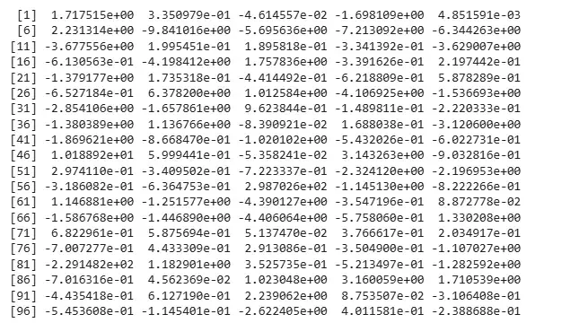
Output

Explanation:

• The output shows random values generated from the Cauchy distribution using rcauchy(100).
• Cauchy distribution has no defined mean or variance, so values can be highly spread out and unstable.
• Some values (like 298.70 and -229.15) are extreme outliers, which is normal for Cauchy.
• Many values are centered near 0, reflecting the location parameter (default is 0).
• The heavy tails make it unsuitable for calculating averages, but useful in robust statistics testing.

10. Fisher-Snedecor Distribution (F-Distribution)

The F-distribution is used to compare variances and in ANOVA. It arises as the ratio of two scaled chi-squared distributions.

**Functions:

• **df(): Probability density function.
• **pf(): Cumulative distribution function.
• **qf(): Quantile function.
• **rf(): Random number generation.

**Example: Generate 100 random values from F-distribution with df1 = 5 and df2 = 10.

R `

random_fisher <- rf(100, df1 = 5, df2 = 10) print(random_fisher)

`

**Output:

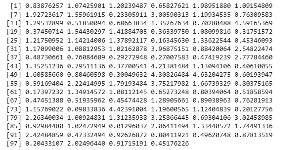
Output

Explanation:

• These are 100 random values generated from an F-distribution using rf().
• Most values lie between 0.2 to 2.5, showing the asymmetry of the F-distribution.
• Some values like 4.63, 4.42 and 4.21 are right-skewed outliers, which is typical in F-distribution.
• Values closer to 1 (e.g., 1.09, 1.29, 1.13) are most common, as expected when group variances are similar.
• Very low (0.01) and very high values show the long tails of the distribution.
• This distribution is mainly used in variance ratio tests, like ANOVA.

11. Dirichlet Distribution

The Dirichlet distribution is a multivariate generalization of the beta distribution. It’s commonly used as a prior in Bayesian statistics for multinomial distributions.

**Functions:

• **rdirichlet(): Random number generation

**Example: Generate 5 samples from a Dirichlet distribution with parameters (1,2,3).

R `

install.packages("MCMCpack") library(MCMCpack) random_dirichlet <- rdirichlet(5, c(1, 2, 3)) print(random_dirichlet)

`

**Output:

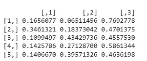
Output

Explanation:

The output shows samples drawn from the Dirichlet distribution. Each row represents one sample and each column corresponds to a component of the distribution based on the given parameters (1, 2, 3).

• Each row contains values between 0 and 1
• The values in each row sum to 1
• These values represent proportions or probabilities across categories.