Version 0.20.1 (May 5, 2017) — pandas 3.0.0.dev0+2100.gf496acffcc documentation (original) (raw)
This is a major release from 0.19.2 and includes a number of API changes, deprecations, new features, enhancements, and performance improvements along with a large number of bug fixes. We recommend that all users upgrade to this version.
Highlights include:
- New
.agg()API for Series/DataFrame similar to the groupby-rolling-resample API’s, see here - Integration with the
feather-format, including a new top-levelpd.read_feather()andDataFrame.to_feather()method, see here. - The
.ixindexer has been deprecated, see here Panelhas been deprecated, see here- Addition of an
IntervalIndexandIntervalscalar type, see here - Improved user API when grouping by index levels in
.groupby(), see here - Improved support for
UInt64dtypes, see here - A new orient for JSON serialization,
orient='table', that uses the Table Schema spec and that gives the possibility for a more interactive repr in the Jupyter Notebook, see here - Experimental support for exporting styled DataFrames (
DataFrame.style) to Excel, see here - Window binary corr/cov operations now return a MultiIndexed
DataFramerather than aPanel, asPanelis now deprecated, see here - Support for S3 handling now uses
s3fs, see here - Google BigQuery support now uses the
pandas-gbqlibrary, see here
Warning
pandas has changed the internal structure and layout of the code base. This can affect imports that are not from the top-level pandas.* namespace, please see the changes here.
Check the API Changes and deprecations before updating.
Note
This is a combined release for 0.20.0 and 0.20.1. Version 0.20.1 contains one additional change for backwards-compatibility with downstream projects using pandas’ utils routines. (GH 16250)
What’s new in v0.20.0
- New features
- Method agg API for DataFrame/Series
- Keyword argument dtype for data IO
- Method .to_datetime() has gained an origin parameter
- GroupBy enhancements
- Better support for compressed URLs in read_csv
- Pickle file IO now supports compression
- UInt64 support improved
- GroupBy on categoricals
- Table schema output
- SciPy sparse matrix from/to SparseDataFrame
- Excel output for styled DataFrames
- IntervalIndex
- Other enhancements
- Backwards incompatible API changes
- Possible incompatibility for HDF5 formats created with pandas < 0.13.0
- Map on Index types now return other Index types
- Accessing datetime fields of Index now return Index
- pd.unique will now be consistent with extension types
- S3 file handling
- Partial string indexing changes
- Concat of different float dtypes will not automatically upcast
- pandas Google BigQuery support has moved
- Memory usage for Index is more accurate
- DataFrame.sort_index changes
- GroupBy describe formatting
- Window binary corr/cov operations return a MultiIndex DataFrame
- HDFStore where string comparison
- Index.intersection and inner join now preserve the order of the left Index
- Pivot table always returns a DataFrame
- Other API changes
- Reorganization of the library: privacy changes
- Deprecations
- Removal of prior version deprecations/changes
- Performance improvements
- Bug fixes
- Contributors
New features#
Method agg API for DataFrame/Series#
Series & DataFrame have been enhanced to support the aggregation API. This is a familiar API from groupby, window operations, and resampling. This allows aggregation operations in a concise way by using agg() and transform(). The full documentation is here (GH 1623).
Here is a sample
In [1]: df = pd.DataFrame(np.random.randn(10, 3), columns=['A', 'B', 'C'], ...: index=pd.date_range('1/1/2000', periods=10)) ...:
In [2]: df.iloc[3:7] = np.nan
In [3]: df Out[3]: A B C 2000-01-01 0.469112 -0.282863 -1.509059 2000-01-02 -1.135632 1.212112 -0.173215 2000-01-03 0.119209 -1.044236 -0.861849 2000-01-04 NaN NaN NaN 2000-01-05 NaN NaN NaN 2000-01-06 NaN NaN NaN 2000-01-07 NaN NaN NaN 2000-01-08 0.113648 -1.478427 0.524988 2000-01-09 0.404705 0.577046 -1.715002 2000-01-10 -1.039268 -0.370647 -1.157892
[10 rows x 3 columns]
One can operate using string function names, callables, lists, or dictionaries of these.
Using a single function is equivalent to .apply.
In [4]: df.agg('sum') Out[4]: A -1.068226 B -1.387015 C -4.892029 Length: 3, dtype: float64
Multiple aggregations with a list of functions.
In [5]: df.agg(['sum', 'min']) Out[5]: A B C sum -1.068226 -1.387015 -4.892029 min -1.135632 -1.478427 -1.715002
[2 rows x 3 columns]
Using a dict provides the ability to apply specific aggregations per column. You will get a matrix-like output of all of the aggregators. The output has one column per unique function. Those functions applied to a particular column will be NaN:
In [6]: df.agg({'A': ['sum', 'min'], 'B': ['min', 'max']}) Out[6]: A B sum -1.068226 NaN min -1.135632 -1.478427 max NaN 1.212112
[3 rows x 2 columns]
The API also supports a .transform() function for broadcasting results.
In [7]: df.transform(['abs', lambda x: x - x.min()])
Out[7]:
A B C
abs abs abs
2000-01-01 0.469112 1.604745 0.282863 1.195563 1.509059 0.205944
2000-01-02 1.135632 0.000000 1.212112 2.690539 0.173215 1.541787
2000-01-03 0.119209 1.254841 1.044236 0.434191 0.861849 0.853153
2000-01-04 NaN NaN NaN NaN NaN NaN
2000-01-05 NaN NaN NaN NaN NaN NaN
2000-01-06 NaN NaN NaN NaN NaN NaN
2000-01-07 NaN NaN NaN NaN NaN NaN
2000-01-08 0.113648 1.249281 1.478427 0.000000 0.524988 2.239990
2000-01-09 0.404705 1.540338 0.577046 2.055473 1.715002 0.000000
2000-01-10 1.039268 0.096364 0.370647 1.107780 1.157892 0.557110
[10 rows x 6 columns]
When presented with mixed dtypes that cannot be aggregated, .agg() will only take the valid aggregations. This is similar to how groupby .agg() works. (GH 15015)
In [8]: df = pd.DataFrame({'A': [1, 2, 3], ...: 'B': [1., 2., 3.], ...: 'C': ['foo', 'bar', 'baz'], ...: 'D': pd.date_range('20130101', periods=3)}) ...:
In [9]: df.dtypes Out[9]: A int64 B float64 C object D datetime64[ns] Length: 4, dtype: object
In [10]: df.agg(['min', 'sum']) Out[10]: A B C D min 1 1.0 bar 2013-01-01 sum 6 6.0 foobarbaz NaT
Keyword argument dtype for data IO#
The 'python' engine for read_csv(), as well as the read_fwf() function for parsing fixed-width text files and read_excel() for parsing Excel files, now accept the dtype keyword argument for specifying the types of specific columns (GH 14295). See the io docs for more information.
In [10]: data = "a b\n1 2\n3 4"
In [11]: pd.read_fwf(StringIO(data)).dtypes Out[11]: a int64 b int64 Length: 2, dtype: object
In [12]: pd.read_fwf(StringIO(data), dtype={'a': 'float64', 'b': 'object'}).dtypes Out[12]: a float64 b object Length: 2, dtype: object
Method .to_datetime() has gained an origin parameter#
to_datetime() has gained a new parameter, origin, to define a reference date from where to compute the resulting timestamps when parsing numerical values with a specific unit specified. (GH 11276, GH 11745)
For example, with 1960-01-01 as the starting date:
In [13]: pd.to_datetime([1, 2, 3], unit='D', origin=pd.Timestamp('1960-01-01')) Out[13]: DatetimeIndex(['1960-01-02', '1960-01-03', '1960-01-04'], dtype='datetime64[ns]', freq=None)
The default is set at origin='unix', which defaults to 1970-01-01 00:00:00, which is commonly called ‘unix epoch’ or POSIX time. This was the previous default, so this is a backward compatible change.
In [14]: pd.to_datetime([1, 2, 3], unit='D') Out[14]: DatetimeIndex(['1970-01-02', '1970-01-03', '1970-01-04'], dtype='datetime64[ns]', freq=None)
GroupBy enhancements#
Strings passed to DataFrame.groupby() as the by parameter may now reference either column names or index level names. Previously, only column names could be referenced. This allows to easily group by a column and index level at the same time. (GH 5677)
In [15]: arrays = [['bar', 'bar', 'baz', 'baz', 'foo', 'foo', 'qux', 'qux'], ....: ['one', 'two', 'one', 'two', 'one', 'two', 'one', 'two']] ....:
In [16]: index = pd.MultiIndex.from_arrays(arrays, names=['first', 'second'])
In [17]: df = pd.DataFrame({'A': [1, 1, 1, 1, 2, 2, 3, 3], ....: 'B': np.arange(8)}, ....: index=index) ....:
In [18]: df
Out[18]:
A B
first second
bar one 1 0
two 1 1
baz one 1 2
two 1 3
foo one 2 4
two 2 5
qux one 3 6
two 3 7
[8 rows x 2 columns]
In [19]: df.groupby(['second', 'A']).sum()
Out[19]:
B
second A
one 1 2
2 4
3 6
two 1 4
2 5
3 7
[6 rows x 1 columns]
Better support for compressed URLs in read_csv#
The compression code was refactored (GH 12688). As a result, reading dataframes from URLs in read_csv() or read_table() now supports additional compression methods: xz, bz2, and zip (GH 14570). Previously, only gzip compression was supported. By default, compression of URLs and paths are now inferred using their file extensions. Additionally, support for bz2 compression in the python 2 C-engine improved (GH 14874).
In [20]: url = ('https://github.com/{repo}/raw/{branch}/{path}' ....: .format(repo='pandas-dev/pandas', ....: branch='main', ....: path='pandas/tests/io/parser/data/salaries.csv.bz2')) ....:
default, infer compression
In [21]: df = pd.read_csv(url, sep='\t', compression='infer')
explicitly specify compression
In [22]: df = pd.read_csv(url, sep='\t', compression='bz2')
In [23]: df.head(2) Out[23]: S X E M 0 13876 1 1 1 1 11608 1 3 0
[2 rows x 4 columns]
Pickle file IO now supports compression#
read_pickle(), DataFrame.to_pickle() and Series.to_pickle()can now read from and write to compressed pickle files. Compression methods can be an explicit parameter or be inferred from the file extension. See the docs here.
In [24]: df = pd.DataFrame({'A': np.random.randn(1000), ....: 'B': 'foo', ....: 'C': pd.date_range('20130101', periods=1000, freq='s')}) ....:
Using an explicit compression type
In [25]: df.to_pickle("data.pkl.compress", compression="gzip")
In [26]: rt = pd.read_pickle("data.pkl.compress", compression="gzip")
In [27]: rt.head() Out[27]: A B C 0 -1.344312 foo 2013-01-01 00:00:00 1 0.844885 foo 2013-01-01 00:00:01 2 1.075770 foo 2013-01-01 00:00:02 3 -0.109050 foo 2013-01-01 00:00:03 4 1.643563 foo 2013-01-01 00:00:04
[5 rows x 3 columns]
The default is to infer the compression type from the extension (compression='infer'):
In [28]: df.to_pickle("data.pkl.gz")
In [29]: rt = pd.read_pickle("data.pkl.gz")
In [30]: rt.head() Out[30]: A B C 0 -1.344312 foo 2013-01-01 00:00:00 1 0.844885 foo 2013-01-01 00:00:01 2 1.075770 foo 2013-01-01 00:00:02 3 -0.109050 foo 2013-01-01 00:00:03 4 1.643563 foo 2013-01-01 00:00:04
[5 rows x 3 columns]
In [31]: df["A"].to_pickle("s1.pkl.bz2")
In [32]: rt = pd.read_pickle("s1.pkl.bz2")
In [33]: rt.head() Out[33]: 0 -1.344312 1 0.844885 2 1.075770 3 -0.109050 4 1.643563 Name: A, Length: 5, dtype: float64
UInt64 support improved#
pandas has significantly improved support for operations involving unsigned, or purely non-negative, integers. Previously, handling these integers would result in improper rounding or data-type casting, leading to incorrect results. Notably, a new numerical index, UInt64Index, has been created (GH 14937)
In [1]: idx = pd.UInt64Index([1, 2, 3]) In [2]: df = pd.DataFrame({'A': ['a', 'b', 'c']}, index=idx) In [3]: df.index Out[3]: UInt64Index([1, 2, 3], dtype='uint64')
- Bug in converting object elements of array-like objects to unsigned 64-bit integers (GH 4471, GH 14982)
- Bug in
Series.unique()in which unsigned 64-bit integers were causing overflow (GH 14721) - Bug in
DataFrameconstruction in which unsigned 64-bit integer elements were being converted to objects (GH 14881) - Bug in
pd.read_csv()in which unsigned 64-bit integer elements were being improperly converted to the wrong data types (GH 14983) - Bug in
pd.unique()in which unsigned 64-bit integers were causing overflow (GH 14915) - Bug in
pd.value_counts()in which unsigned 64-bit integers were being erroneously truncated in the output (GH 14934)
GroupBy on categoricals#
In previous versions, .groupby(..., sort=False) would fail with a ValueError when grouping on a categorical series with some categories not appearing in the data. (GH 13179)
In [34]: chromosomes = np.r_[np.arange(1, 23).astype(str), ['X', 'Y']]
In [35]: df = pd.DataFrame({ ....: 'A': np.random.randint(100), ....: 'B': np.random.randint(100), ....: 'C': np.random.randint(100), ....: 'chromosomes': pd.Categorical(np.random.choice(chromosomes, 100), ....: categories=chromosomes, ....: ordered=True)}) ....:
In [36]: df Out[36]: A B C chromosomes 0 87 22 81 4 1 87 22 81 13 2 87 22 81 22 3 87 22 81 2 4 87 22 81 6 .. .. .. .. ... 95 87 22 81 8 96 87 22 81 11 97 87 22 81 X 98 87 22 81 1 99 87 22 81 19
[100 rows x 4 columns]
Previous behavior:
In [3]: df[df.chromosomes != '1'].groupby('chromosomes', observed=False, sort=False).sum()
ValueError: items in new_categories are not the same as in old categories
New behavior:
In [37]: df[df.chromosomes != '1'].groupby('chromosomes', observed=False, sort=False).sum()
Out[37]:
A B C
chromosomes
4 348 88 324
13 261 66 243
22 348 88 324
2 348 88 324
6 174 44 162
... ... .. ...
3 348 88 324
11 348 88 324
19 174 44 162
1 0 0 0
21 0 0 0
[24 rows x 3 columns]
Table schema output#
The new orient 'table' for DataFrame.to_json()will generate a Table Schema compatible string representation of the data.
In [38]: df = pd.DataFrame( ....: {'A': [1, 2, 3], ....: 'B': ['a', 'b', 'c'], ....: 'C': pd.date_range('2016-01-01', freq='d', periods=3)}, ....: index=pd.Index(range(3), name='idx')) In [39]: df Out[39]: A B C idx 0 1 a 2016-01-01 1 2 b 2016-01-02 2 3 c 2016-01-03
[3 rows x 3 columns]
In [40]: df.to_json(orient='table') Out[40]: '{"schema":{"fields":[{"name":"idx","type":"integer"},{"name":"A","type":"integer"},{"name":"B","type":"string"},{"name":"C","type":"datetime"}],"primaryKey":["idx"],"pandas_version":"1.4.0"},"data":[{"idx":0,"A":1,"B":"a","C":"2016-01-01T00:00:00.000"},{"idx":1,"A":2,"B":"b","C":"2016-01-02T00:00:00.000"},{"idx":2,"A":3,"B":"c","C":"2016-01-03T00:00:00.000"}]}'
See IO: Table Schema for more information.
Additionally, the repr for DataFrame and Series can now publish this JSON Table schema representation of the Series or DataFrame if you are using IPython (or another frontend like nteract using the Jupyter messaging protocol). This gives frontends like the Jupyter notebook and nteractmore flexibility in how they display pandas objects, since they have more information about the data. You must enable this by setting the display.html.table_schema option to True.
SciPy sparse matrix from/to SparseDataFrame#
pandas now supports creating sparse dataframes directly from scipy.sparse.spmatrix instances. See the documentation for more information. (GH 4343)
All sparse formats are supported, but matrices that are not in COOrdinate format will be converted, copying data as needed.
from scipy.sparse import csr_matrix arr = np.random.random(size=(1000, 5)) arr[arr < .9] = 0 sp_arr = csr_matrix(arr) sp_arr sdf = pd.SparseDataFrame(sp_arr) sdf
To convert a SparseDataFrame back to sparse SciPy matrix in COO format, you can use:
Excel output for styled DataFrames#
Experimental support has been added to export DataFrame.style formats to Excel using the openpyxl engine. (GH 15530)
For example, after running the following, styled.xlsx renders as below:
In [38]: np.random.seed(24)
In [39]: df = pd.DataFrame({'A': np.linspace(1, 10, 10)})
In [40]: df = pd.concat([df, pd.DataFrame(np.random.RandomState(24).randn(10, 4), ....: columns=list('BCDE'))], ....: axis=1) ....:
In [41]: df.iloc[0, 2] = np.nan
In [42]: df Out[42]: A B C D E 0 1.0 1.329212 NaN -0.316280 -0.990810 1 2.0 -1.070816 -1.438713 0.564417 0.295722 2 3.0 -1.626404 0.219565 0.678805 1.889273 3 4.0 0.961538 0.104011 -0.481165 0.850229 4 5.0 1.453425 1.057737 0.165562 0.515018 5 6.0 -1.336936 0.562861 1.392855 -0.063328 6 7.0 0.121668 1.207603 -0.002040 1.627796 7 8.0 0.354493 1.037528 -0.385684 0.519818 8 9.0 1.686583 -1.325963 1.428984 -2.089354 9 10.0 -0.129820 0.631523 -0.586538 0.290720
[10 rows x 5 columns]
In [43]: styled = (df.style ....: .map(lambda val: 'color:red;' if val < 0 else 'color:black;') ....: .highlight_max()) ....:
In [44]: styled.to_excel('styled.xlsx', engine='openpyxl')
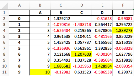
See the Style documentation for more detail.
IntervalIndex#
pandas has gained an IntervalIndex with its own dtype, interval as well as the Interval scalar type. These allow first-class support for interval notation, specifically as a return type for the categories in cut() and qcut(). The IntervalIndex allows some unique indexing, see thedocs. (GH 7640, GH 8625)
Warning
These indexing behaviors of the IntervalIndex are provisional and may change in a future version of pandas. Feedback on usage is welcome.
Previous behavior:
The returned categories were strings, representing Intervals
In [1]: c = pd.cut(range(4), bins=2)
In [2]: c Out[2]: [(-0.003, 1.5], (-0.003, 1.5], (1.5, 3], (1.5, 3]] Categories (2, object): [(-0.003, 1.5] < (1.5, 3]]
In [3]: c.categories Out[3]: Index(['(-0.003, 1.5]', '(1.5, 3]'], dtype='object')
New behavior:
In [45]: c = pd.cut(range(4), bins=2)
In [46]: c Out[46]: [(-0.003, 1.5], (-0.003, 1.5], (1.5, 3.0], (1.5, 3.0]] Categories (2, interval[float64, right]): [(-0.003, 1.5] < (1.5, 3.0]]
In [47]: c.categories Out[47]: IntervalIndex([(-0.003, 1.5], (1.5, 3.0]], dtype='interval[float64, right]')
Furthermore, this allows one to bin other data with these same bins, with NaN representing a missing value similar to other dtypes.
In [48]: pd.cut([0, 3, 5, 1], bins=c.categories) Out[48]: [(-0.003, 1.5], (1.5, 3.0], NaN, (-0.003, 1.5]] Categories (2, interval[float64, right]): [(-0.003, 1.5] < (1.5, 3.0]]
An IntervalIndex can also be used in Series and DataFrame as the index.
In [49]: df = pd.DataFrame({'A': range(4), ....: 'B': pd.cut([0, 3, 1, 1], bins=c.categories) ....: }).set_index('B') ....:
In [50]: df
Out[50]:
A
B
(-0.003, 1.5] 0
(1.5, 3.0] 1
(-0.003, 1.5] 2
(-0.003, 1.5] 3
[4 rows x 1 columns]
Selecting via a specific interval:
In [51]: df.loc[pd.Interval(1.5, 3.0)] Out[51]: A 1 Name: (1.5, 3.0], Length: 1, dtype: int64
Selecting via a scalar value that is contained in the intervals.
In [52]: df.loc[0]
Out[52]:
A
B
(-0.003, 1.5] 0
(-0.003, 1.5] 2
(-0.003, 1.5] 3
[3 rows x 1 columns]
Other enhancements#
DataFrame.rolling()now accepts the parameterclosed='right'|'left'|'both'|'neither'to choose the rolling window-endpoint closedness. See the documentation (GH 13965)- Integration with the
feather-format, including a new top-levelpd.read_feather()andDataFrame.to_feather()method, see here. Series.str.replace()now accepts a callable, as replacement, which is passed tore.sub(GH 15055)Series.str.replace()now accepts a compiled regular expression as a pattern (GH 15446)Series.sort_indexaccepts parameterskindandna_position(GH 13589, GH 14444)DataFrameandDataFrame.groupby()have gained anunique()method to count the distinct values over an axis (GH 14336, GH 15197).DataFramehas gained amelt()method, equivalent topd.melt(), for unpivoting from a wide to long format (GH 12640).pd.read_excel()now preserves sheet order when usingsheetname=None(GH 9930)- Multiple offset aliases with decimal points are now supported (e.g.
0.5minis parsed as30s) (GH 8419) .isnull()and.notnull()have been added toIndexobject to make them more consistent with theSeriesAPI (GH 15300)- New
UnsortedIndexError(subclass ofKeyError) raised when indexing/slicing into an unsorted MultiIndex (GH 11897). This allows differentiation between errors due to lack of sorting or an incorrect key. See here MultiIndexhas gained a.to_frame()method to convert to aDataFrame(GH 12397)pd.cutandpd.qcutnow support datetime64 and timedelta64 dtypes (GH 14714, GH 14798)pd.qcuthas gained theduplicates='raise'|'drop'option to control whether to raise on duplicated edges (GH 7751)Seriesprovides ato_excelmethod to output Excel files (GH 8825)- The
usecolsargument inpd.read_csv()now accepts a callable function as a value (GH 14154) - The
skiprowsargument inpd.read_csv()now accepts a callable function as a value (GH 10882) - The
nrowsandchunksizearguments inpd.read_csv()are supported if both are passed (GH 6774, GH 15755) DataFrame.plotnow prints a title above each subplot ifsuplots=Trueandtitleis a list of strings (GH 14753)DataFrame.plotcan pass the matplotlib 2.0 default color cycle as a single string as color parameter, see here. (GH 15516)Series.interpolate()now supports timedelta as an index type withmethod='time'(GH 6424)- Addition of a
levelkeyword toDataFrame/Series.renameto rename labels in the specified level of a MultiIndex (GH 4160). DataFrame.reset_index()will now interpret a tupleindex.nameas a key spanning across levels ofcolumns, if this is aMultiIndex(GH 16164)Timedelta.isoformatmethod added for formatting Timedeltas as an ISO 8601 duration. See the Timedelta docs (GH 15136).select_dtypes()now allows the stringdatetimetzto generically select datetimes with tz (GH 14910)- The
.to_latex()method will now acceptmulticolumnandmultirowarguments to use the accompanying LaTeX enhancements pd.merge_asof()gained the optiondirection='backward'|'forward'|'nearest'(GH 14887)Series/DataFrame.asfreq()have gained afill_valueparameter, to fill missing values (GH 3715).Series/DataFrame.resample.asfreqhave gained afill_valueparameter, to fill missing values during resampling (GH 3715).- pandas.util.hash_pandas_object() has gained the ability to hash a
MultiIndex(GH 15224) Series/DataFrame.squeeze()have gained theaxisparameter. (GH 15339)DataFrame.to_excel()has a newfreeze_panesparameter to turn on Freeze Panes when exporting to Excel (GH 15160)pd.read_html()will parse multiple header rows, creating a MultiIndex header. (GH 13434).- HTML table output skips
colspanorrowspanattribute if equal to 1. (GH 15403) - pandas.io.formats.style.Styler template now has blocks for easier extension, see the example notebook (GH 15649)
Styler.render()now accepts**kwargsto allow user-defined variables in the template (GH 15649)- Compatibility with Jupyter notebook 5.0; MultiIndex column labels are left-aligned and MultiIndex row-labels are top-aligned (GH 15379)
TimedeltaIndexnow has a custom date-tick formatter specifically designed for nanosecond level precision (GH 8711)pd.api.types.union_categoricalsgained theignore_orderedargument to allow ignoring the ordered attribute of unioned categoricals (GH 13410). See the categorical union docs for more information.DataFrame.to_latex()andDataFrame.to_string()now allow optional header aliases. (GH 15536)- Re-enable the
parse_dateskeyword ofpd.read_excel()to parse string columns as dates (GH 14326) - Added
.emptyproperty to subclasses ofIndex. (GH 15270) - Enabled floor division for
TimedeltaandTimedeltaIndex(GH 15828) pandas.io.json.json_normalize()gained the optionerrors='ignore'|'raise'; the default iserrors='raise'which is backward compatible. (GH 14583)pandas.io.json.json_normalize()with an emptylistwill return an emptyDataFrame(GH 15534)pandas.io.json.json_normalize()has gained asepoption that acceptsstrto separate joined fields; the default is “.”, which is backward compatible. (GH 14883)- MultiIndex.remove_unused_levels() has been added to facilitate removing unused levels. (GH 15694)
pd.read_csv()will now raise aParserErrorerror whenever any parsing error occurs (GH 15913, GH 15925)pd.read_csv()now supports theerror_bad_linesandwarn_bad_linesarguments for the Python parser (GH 15925)- The
display.show_dimensionsoption can now also be used to specify whether the length of aSeriesshould be shown in its repr (GH 7117). parallel_coordinates()has gained asort_labelskeyword argument that sorts class labels and the colors assigned to them (GH 15908)- Options added to allow one to turn on/off using
bottleneckandnumexpr, see here (GH 16157) DataFrame.style.bar()now accepts two more options to further customize the bar chart. Bar alignment is set withalign='left'|'mid'|'zero', the default is “left”, which is backward compatible; You can now pass a list ofcolor=[color_negative, color_positive]. (GH 14757)
Backwards incompatible API changes#
Possible incompatibility for HDF5 formats created with pandas < 0.13.0#
pd.TimeSeries was deprecated officially in 0.17.0, though has already been an alias since 0.13.0. It has been dropped in favor of pd.Series. (GH 15098).
This may cause HDF5 files that were created in prior versions to become unreadable if pd.TimeSerieswas used. This is most likely to be for pandas < 0.13.0. If you find yourself in this situation. You can use a recent prior version of pandas to read in your HDF5 files, then write them out again after applying the procedure below.
In [2]: s = pd.TimeSeries([1, 2, 3], index=pd.date_range('20130101', periods=3))
In [3]: s Out[3]: 2013-01-01 1 2013-01-02 2 2013-01-03 3 Freq: D, dtype: int64
In [4]: type(s) Out[4]: pandas.core.series.TimeSeries
In [5]: s = pd.Series(s)
In [6]: s Out[6]: 2013-01-01 1 2013-01-02 2 2013-01-03 3 Freq: D, dtype: int64
In [7]: type(s) Out[7]: pandas.core.series.Series
Map on Index types now return other Index types#
map on an Index now returns an Index, not a numpy array (GH 12766)
In [53]: idx = pd.Index([1, 2])
In [54]: idx Out[54]: Index([1, 2], dtype='int64')
In [55]: mi = pd.MultiIndex.from_tuples([(1, 2), (2, 4)])
In [56]: mi Out[56]: MultiIndex([(1, 2), (2, 4)], )
Previous behavior:
In [5]: idx.map(lambda x: x * 2) Out[5]: array([2, 4])
In [6]: idx.map(lambda x: (x, x * 2)) Out[6]: array([(1, 2), (2, 4)], dtype=object)
In [7]: mi.map(lambda x: x) Out[7]: array([(1, 2), (2, 4)], dtype=object)
In [8]: mi.map(lambda x: x[0]) Out[8]: array([1, 2])
New behavior:
In [57]: idx.map(lambda x: x * 2) Out[57]: Index([2, 4], dtype='int64')
In [58]: idx.map(lambda x: (x, x * 2)) Out[58]: MultiIndex([(1, 2), (2, 4)], )
In [59]: mi.map(lambda x: x) Out[59]: MultiIndex([(1, 2), (2, 4)], )
In [60]: mi.map(lambda x: x[0]) Out[60]: Index([1, 2], dtype='int64')
map on a Series with datetime64 values may return int64 dtypes rather than int32
In [64]: s = pd.Series(pd.date_range('2011-01-02T00:00', '2011-01-02T02:00', freq='H') ....: .tz_localize('Asia/Tokyo')) ....:
In [65]: s Out[65]: 0 2011-01-02 00:00:00+09:00 1 2011-01-02 01:00:00+09:00 2 2011-01-02 02:00:00+09:00 Length: 3, dtype: datetime64[ns, Asia/Tokyo]
Previous behavior:
In [9]: s.map(lambda x: x.hour) Out[9]: 0 0 1 1 2 2 dtype: int32
New behavior:
In [66]: s.map(lambda x: x.hour) Out[66]: 0 0 1 1 2 2 Length: 3, dtype: int64
Accessing datetime fields of Index now return Index#
The datetime-related attributes (see herefor an overview) of DatetimeIndex, PeriodIndex and TimedeltaIndex previously returned numpy arrays. They will now return a new Index object, except in the case of a boolean field, where the result will still be a boolean ndarray. (GH 15022)
Previous behaviour:
In [1]: idx = pd.date_range("2015-01-01", periods=5, freq='10H')
In [2]: idx.hour Out[2]: array([ 0, 10, 20, 6, 16], dtype=int32)
New behavior:
In [67]: idx = pd.date_range("2015-01-01", periods=5, freq='10H')
In [68]: idx.hour Out[68]: Index([0, 10, 20, 6, 16], dtype='int32')
This has the advantage that specific Index methods are still available on the result. On the other hand, this might have backward incompatibilities: e.g. compared to numpy arrays, Index objects are not mutable. To get the original ndarray, you can always convert explicitly using np.asarray(idx.hour).
pd.unique will now be consistent with extension types#
In prior versions, using Series.unique() and pandas.unique() on Categorical and tz-aware data-types would yield different return types. These are now made consistent. (GH 15903)
- Datetime tz-aware
Previous behaviour:
Series
In [5]: pd.Series([pd.Timestamp('20160101', tz='US/Eastern'),
...: pd.Timestamp('20160101', tz='US/Eastern')]).unique()
Out[5]: array([Timestamp('2016-01-01 00:00:00-0500', tz='US/Eastern')], dtype=object)
In [6]: pd.unique(pd.Series([pd.Timestamp('20160101', tz='US/Eastern'),
...: pd.Timestamp('20160101', tz='US/Eastern')]))
Out[6]: array(['2016-01-01T05:00:00.000000000'], dtype='datetime64[ns]')
Index
In [7]: pd.Index([pd.Timestamp('20160101', tz='US/Eastern'),
...: pd.Timestamp('20160101', tz='US/Eastern')]).unique()
Out[7]: DatetimeIndex(['2016-01-01 00:00:00-05:00'], dtype='datetime64[ns, US/Eastern]', freq=None)
In [8]: pd.unique([pd.Timestamp('20160101', tz='US/Eastern'),
...: pd.Timestamp('20160101', tz='US/Eastern')])
Out[8]: array(['2016-01-01T05:00:00.000000000'], dtype='datetime64[ns]')
New behavior:
Series, returns an array of Timestamp tz-aware
In [61]: pd.Series([pd.Timestamp(r'20160101', tz=r'US/Eastern'),
....: pd.Timestamp(r'20160101', tz=r'US/Eastern')]).unique()
....:
Out[61]:
['2016-01-01 00:00:00-05:00']
Length: 1, dtype: datetime64[s, US/Eastern]
In [62]: pd.unique(pd.Series([pd.Timestamp('20160101', tz='US/Eastern'),
....: pd.Timestamp('20160101', tz='US/Eastern')]))
....:
Out[62]:
['2016-01-01 00:00:00-05:00']
Length: 1, dtype: datetime64[s, US/Eastern]
Index, returns a DatetimeIndex
In [63]: pd.Index([pd.Timestamp('20160101', tz='US/Eastern'),
....: pd.Timestamp('20160101', tz='US/Eastern')]).unique()
....:
Out[63]: DatetimeIndex(['2016-01-01 00:00:00-05:00'], dtype='datetime64[s, US/Eastern]', freq=None)
In [64]: pd.unique(pd.Index([pd.Timestamp('20160101', tz='US/Eastern'),
....: pd.Timestamp('20160101', tz='US/Eastern')]))
....:
Out[64]: DatetimeIndex(['2016-01-01 00:00:00-05:00'], dtype='datetime64[s, US/Eastern]', freq=None)
- Categoricals
Previous behaviour:
In [1]: pd.Series(list('baabc'), dtype='category').unique()
Out[1]:
[b, a, c]
Categories (3, object): [b, a, c]
In [2]: pd.unique(pd.Series(list('baabc'), dtype='category'))
Out[2]: array(['b', 'a', 'c'], dtype=object)
New behavior:
returns a Categorical
In [65]: pd.Series(list('baabc'), dtype='category').unique()
Out[65]:
['b', 'a', 'c']
Categories (3, object): ['a', 'b', 'c']
In [66]: pd.unique(pd.Series(list('baabc'), dtype='category'))
Out[66]:
['b', 'a', 'c']
Categories (3, object): ['a', 'b', 'c']
S3 file handling#
pandas now uses s3fs for handling S3 connections. This shouldn’t break any code. However, since s3fs is not a required dependency, you will need to install it separately, like botoin prior versions of pandas. (GH 11915).
Partial string indexing changes#
DatetimeIndex Partial String Indexing now works as an exact match, provided that string resolution coincides with index resolution, including a case when both are seconds (GH 14826). See Slice vs. Exact Match for details.
In [67]: df = pd.DataFrame({'a': [1, 2, 3]}, pd.DatetimeIndex(['2011-12-31 23:59:59', ....: '2012-01-01 00:00:00', ....: '2012-01-01 00:00:01'])) ....:
Previous behavior:
In [4]: df['2011-12-31 23:59:59'] Out[4]: a 2011-12-31 23:59:59 1
In [5]: df['a']['2011-12-31 23:59:59'] Out[5]: 2011-12-31 23:59:59 1 Name: a, dtype: int64
New behavior:
In [4]: df['2011-12-31 23:59:59'] KeyError: '2011-12-31 23:59:59'
In [5]: df['a']['2011-12-31 23:59:59'] Out[5]: 1
Concat of different float dtypes will not automatically upcast#
Previously, concat of multiple objects with different float dtypes would automatically upcast results to a dtype of float64. Now the smallest acceptable dtype will be used (GH 13247)
In [68]: df1 = pd.DataFrame(np.array([1.0], dtype=np.float32, ndmin=2))
In [69]: df1.dtypes Out[69]: 0 float32 Length: 1, dtype: object
In [70]: df2 = pd.DataFrame(np.array([np.nan], dtype=np.float32, ndmin=2))
In [71]: df2.dtypes Out[71]: 0 float32 Length: 1, dtype: object
Previous behavior:
In [7]: pd.concat([df1, df2]).dtypes Out[7]: 0 float64 dtype: object
New behavior:
In [72]: pd.concat([df1, df2]).dtypes Out[72]: 0 float32 Length: 1, dtype: object
pandas Google BigQuery support has moved#
pandas has split off Google BigQuery support into a separate package pandas-gbq. You can conda install pandas-gbq -c conda-forge orpip install pandas-gbq to get it. The functionality of read_gbq() and DataFrame.to_gbq() remain the same with the currently released version of pandas-gbq=0.1.4. Documentation is now hosted here (GH 15347)
Memory usage for Index is more accurate#
In previous versions, showing .memory_usage() on a pandas structure that has an index, would only include actual index values and not include structures that facilitated fast indexing. This will generally be different for Index and MultiIndex and less-so for other index types. (GH 15237)
Previous behavior:
In [8]: index = pd.Index(['foo', 'bar', 'baz'])
In [9]: index.memory_usage(deep=True) Out[9]: 180
In [10]: index.get_loc('foo') Out[10]: 0
In [11]: index.memory_usage(deep=True) Out[11]: 180
New behavior:
In [8]: index = pd.Index(['foo', 'bar', 'baz'])
In [9]: index.memory_usage(deep=True) Out[9]: 180
In [10]: index.get_loc('foo') Out[10]: 0
In [11]: index.memory_usage(deep=True) Out[11]: 260
DataFrame.sort_index changes#
In certain cases, calling .sort_index() on a MultiIndexed DataFrame would return the same DataFrame without seeming to sort. This would happen with a lexsorted, but non-monotonic levels. (GH 15622, GH 15687, GH 14015, GH 13431, GH 15797)
This is unchanged from prior versions, but shown for illustration purposes:
In [81]: df = pd.DataFrame(np.arange(6), columns=['value'], ....: index=pd.MultiIndex.from_product([list('BA'), range(3)])) ....: In [82]: df
Out[82]: value B 0 0 1 1 2 2 A 0 3 1 4 2 5
[6 rows x 1 columns]
In [87]: df.index.is_lexsorted() Out[87]: False
In [88]: df.index.is_monotonic Out[88]: False
Sorting works as expected
In [73]: df.sort_index() Out[73]: a 2011-12-31 23:59:59 1 2012-01-01 00:00:00 2 2012-01-01 00:00:01 3
[3 rows x 1 columns]
In [90]: df.sort_index().index.is_lexsorted() Out[90]: True
In [91]: df.sort_index().index.is_monotonic Out[91]: True
However, this example, which has a non-monotonic 2nd level, doesn’t behave as desired.
In [74]: df = pd.DataFrame({'value': [1, 2, 3, 4]}, ....: index=pd.MultiIndex([['a', 'b'], ['bb', 'aa']], ....: [[0, 0, 1, 1], [0, 1, 0, 1]])) ....:
In [75]: df Out[75]: value a bb 1 aa 2 b bb 3 aa 4
[4 rows x 1 columns]
Previous behavior:
In [11]: df.sort_index() Out[11]: value a bb 1 aa 2 b bb 3 aa 4
In [14]: df.sort_index().index.is_lexsorted() Out[14]: True
In [15]: df.sort_index().index.is_monotonic Out[15]: False
New behavior:
In [94]: df.sort_index() Out[94]: value a aa 2 bb 1 b aa 4 bb 3
[4 rows x 1 columns]
In [95]: df.sort_index().index.is_lexsorted() Out[95]: True
In [96]: df.sort_index().index.is_monotonic Out[96]: True
GroupBy describe formatting#
The output formatting of groupby.describe() now labels the describe() metrics in the columns instead of the index. This format is consistent with groupby.agg() when applying multiple functions at once. (GH 4792)
Previous behavior:
In [1]: df = pd.DataFrame({'A': [1, 1, 2, 2], 'B': [1, 2, 3, 4]})
In [2]: df.groupby('A').describe() Out[2]: B A 1 count 2.000000 mean 1.500000 std 0.707107 min 1.000000 25% 1.250000 50% 1.500000 75% 1.750000 max 2.000000 2 count 2.000000 mean 3.500000 std 0.707107 min 3.000000 25% 3.250000 50% 3.500000 75% 3.750000 max 4.000000
In [3]: df.groupby('A').agg(["mean", "std", "min", "max"]) Out[3]: B mean std amin amax A 1 1.5 0.707107 1 2 2 3.5 0.707107 3 4
New behavior:
In [76]: df = pd.DataFrame({'A': [1, 1, 2, 2], 'B': [1, 2, 3, 4]})
In [77]: df.groupby('A').describe()
Out[77]:
B
count mean std min 25% 50% 75% max
A
1 2.0 1.5 0.707107 1.0 1.25 1.5 1.75 2.0
2 2.0 3.5 0.707107 3.0 3.25 3.5 3.75 4.0
[2 rows x 8 columns]
In [78]: df.groupby('A').agg(["mean", "std", "min", "max"])
Out[78]:
B
mean std min max
A
1 1.5 0.707107 1 2
2 3.5 0.707107 3 4
[2 rows x 4 columns]
Window binary corr/cov operations return a MultiIndex DataFrame#
A binary window operation, like .corr() or .cov(), when operating on a .rolling(..), .expanding(..), or .ewm(..) object, will now return a 2-level MultiIndexed DataFrame rather than a Panel, as Panel is now deprecated, see here. These are equivalent in function, but a MultiIndexed DataFrame enjoys more support in pandas. See the section on Windowed Binary Operations for more information. (GH 15677)
In [79]: np.random.seed(1234)
In [80]: df = pd.DataFrame(np.random.rand(100, 2), ....: columns=pd.Index(['A', 'B'], name='bar'), ....: index=pd.date_range('20160101', ....: periods=100, freq='D', name='foo')) ....:
In [81]: df.tail()
Out[81]:
bar A B
foo
2016-04-05 0.640880 0.126205
2016-04-06 0.171465 0.737086
2016-04-07 0.127029 0.369650
2016-04-08 0.604334 0.103104
2016-04-09 0.802374 0.945553
[5 rows x 2 columns]
Previous behavior:
In [2]: df.rolling(12).corr() Out[2]: <class 'pandas.core.panel.Panel'> Dimensions: 100 (items) x 2 (major_axis) x 2 (minor_axis) Items axis: 2016-01-01 00:00:00 to 2016-04-09 00:00:00 Major_axis axis: A to B Minor_axis axis: A to B
New behavior:
In [82]: res = df.rolling(12).corr()
In [83]: res.tail()
Out[83]:
bar A B
foo bar
2016-04-07 B -0.132090 1.000000
2016-04-08 A 1.000000 -0.145775
B -0.145775 1.000000
2016-04-09 A 1.000000 0.119645
B 0.119645 1.000000
[5 rows x 2 columns]
Retrieving a correlation matrix for a cross-section
In [84]: df.rolling(12).corr().loc['2016-04-07']
Out[84]:
bar A B
bar
A 1.00000 -0.13209
B -0.13209 1.00000
[2 rows x 2 columns]
HDFStore where string comparison#
In previous versions most types could be compared to string column in a HDFStoreusually resulting in an invalid comparison, returning an empty result frame. These comparisons will now raise aTypeError (GH 15492)
In [85]: df = pd.DataFrame({'unparsed_date': ['2014-01-01', '2014-01-01']})
In [86]: df.to_hdf('store.h5', key='key', format='table', data_columns=True)
In [87]: df.dtypes Out[87]: unparsed_date object Length: 1, dtype: object
Previous behavior:
In [4]: pd.read_hdf('store.h5', 'key', where='unparsed_date > ts') File "", line 1 (unparsed_date > 1970-01-01 00:00:01.388552400) ^ SyntaxError: invalid token
New behavior:
In [18]: ts = pd.Timestamp('2014-01-01')
In [19]: pd.read_hdf('store.h5', 'key', where='unparsed_date > ts') TypeError: Cannot compare 2014-01-01 00:00:00 of type <class 'pandas.tslib.Timestamp'> to string column
Index.intersection and inner join now preserve the order of the left Index#
Index.intersection() now preserves the order of the calling Index (left) instead of the other Index (right) (GH 15582). This affects inner joins, DataFrame.join() and merge(), and the .align method.
Index.intersection
In [88]: left = pd.Index([2, 1, 0])
In [89]: left
Out[89]: Index([2, 1, 0], dtype='int64')
In [90]: right = pd.Index([1, 2, 3])
In [91]: right
Out[91]: Index([1, 2, 3], dtype='int64')
Previous behavior:
In [4]: left.intersection(right)
Out[4]: Int64Index([1, 2], dtype='int64')
New behavior:
In [92]: left.intersection(right)
Out[92]: Index([2, 1], dtype='int64')DataFrame.joinandpd.merge
In [93]: left = pd.DataFrame({'a': [20, 10, 0]}, index=[2, 1, 0])
In [94]: left
Out[94]:
a
2 20
1 10
0 0
[3 rows x 1 columns]
In [95]: right = pd.DataFrame({'b': [100, 200, 300]}, index=[1, 2, 3])
In [96]: right
Out[96]:
b
1 100
2 200
3 300
[3 rows x 1 columns]
Previous behavior:
In [4]: left.join(right, how='inner')
Out[4]:
a b
1 10 100
2 20 200
New behavior:
In [97]: left.join(right, how='inner')
Out[97]:
a b
2 20 200
1 10 100
[2 rows x 2 columns]
Pivot table always returns a DataFrame#
The documentation for pivot_table() states that a DataFrame is always returned. Here a bug is fixed that allowed this to return a Series under certain circumstance. (GH 4386)
In [98]: df = pd.DataFrame({'col1': [3, 4, 5], ....: 'col2': ['C', 'D', 'E'], ....: 'col3': [1, 3, 9]}) ....:
In [99]: df Out[99]: col1 col2 col3 0 3 C 1 1 4 D 3 2 5 E 9
[3 rows x 3 columns]
Previous behavior:
In [2]: df.pivot_table('col1', index=['col3', 'col2'], aggfunc="sum") Out[2]: col3 col2 1 C 3 3 D 4 9 E 5 Name: col1, dtype: int64
New behavior:
In [100]: df.pivot_table('col1', index=['col3', 'col2'], aggfunc="sum")
Out[100]:
col1
col3 col2
1 C 3
3 D 4
9 E 5
[3 rows x 1 columns]
Other API changes#
numexprversion is now required to be >= 2.4.6 and it will not be used at all if this requisite is not fulfilled (GH 15213).CParserErrorhas been renamed toParserErrorinpd.read_csv()and will be removed in the future (GH 12665)SparseArray.cumsum()andSparseSeries.cumsum()will now always returnSparseArrayandSparseSeriesrespectively (GH 12855)DataFrame.applymap()with an emptyDataFramewill return a copy of the emptyDataFrameinstead of aSeries(GH 8222)Series.map()now respects default values of dictionary subclasses with a__missing__method, such ascollections.Counter(GH 15999).lochas compat with.ixfor accepting iterators, and NamedTuples (GH 15120)interpolate()andfillna()will raise aValueErrorif thelimitkeyword argument is not greater than 0. (GH 9217)pd.read_csv()will now issue aParserWarningwhenever there are conflicting values provided by thedialectparameter and the user (GH 14898)pd.read_csv()will now raise aValueErrorfor the C engine if the quote character is larger than one byte (GH 11592)inplacearguments now require a boolean value, else aValueErroris thrown (GH 14189)pandas.api.types.is_datetime64_ns_dtypewill now reportTrueon a tz-aware dtype, similar topandas.api.types.is_datetime64_any_dtypeDataFrame.asof()will return a null filledSeriesinstead the scalarNaNif a match is not found (GH 15118)- Specific support for
copy.copy()andcopy.deepcopy()functions on NDFrame objects (GH 15444) Series.sort_values()accepts a one element list of bool for consistency with the behavior ofDataFrame.sort_values()(GH 15604).merge()and.join()oncategorydtype columns will now preserve the category dtype when possible (GH 10409)SparseDataFrame.default_fill_valuewill be 0, previously wasnanin the return frompd.get_dummies(..., sparse=True)(GH 15594)- The default behaviour of
Series.str.matchhas changed from extracting groups to matching the pattern. The extracting behaviour was deprecated since pandas version 0.13.0 and can be done with theSeries.str.extractmethod (GH 5224). As a consequence, theas_indexerkeyword is ignored (no longer needed to specify the new behaviour) and is deprecated. NaTwill now correctly reportFalsefor datetimelike boolean operations such asis_month_start(GH 15781)NaTwill now correctly returnnp.nanforTimedeltaandPeriodaccessors such asdaysandquarter(GH 15782)NaTwill now returnsNaTfortz_localizeandtz_convertmethods (GH 15830)DataFrameandPanelconstructors with invalid input will now raiseValueErrorrather thanPandasError, if called with scalar inputs and not axes (GH 15541)DataFrameandPanelconstructors with invalid input will now raiseValueErrorrather thanpandas.core.common.PandasError, if called with scalar inputs and not axes; The exceptionPandasErroris removed as well. (GH 15541)- The exception
pandas.core.common.AmbiguousIndexErroris removed as it is not referenced (GH 15541)
Reorganization of the library: privacy changes#
Modules privacy has changed#
Some formerly public python/c/c++/cython extension modules have been moved and/or renamed. These are all removed from the public API. Furthermore, the pandas.core, pandas.compat, and pandas.util top-level modules are now considered to be PRIVATE. If indicated, a deprecation warning will be issued if you reference these modules. (GH 12588)
Some new subpackages are created with public functionality that is not directly exposed in the top-level namespace: pandas.errors, pandas.plotting andpandas.testing (more details below). Together with pandas.api.types and certain functions in the pandas.io and pandas.tseries submodules, these are now the public subpackages.
Further changes:
- The function union_categoricals() is now importable from
pandas.api.types, formerly frompandas.types.concat(GH 15998) - The type import
pandas.tslib.NaTTypeis deprecated and can be replaced by usingtype(pandas.NaT)(GH 16146) - The public functions in
pandas.tools.hashingdeprecated from that locations, but are now importable frompandas.util(GH 16223) - The modules in
pandas.util:decorators,print_versions,doctools,validators,depr_moduleare now private. Only the functions exposed inpandas.utilitself are public (GH 16223)
pandas.errors#
We are adding a standard public module for all pandas exceptions & warnings pandas.errors. (GH 14800). Previously these exceptions & warnings could be imported from pandas.core.common or pandas.io.common. These exceptions and warnings will be removed from the *.common locations in a future release. (GH 15541)
The following are now part of this API:
['DtypeWarning', 'EmptyDataError', 'OutOfBoundsDatetime', 'ParserError', 'ParserWarning', 'PerformanceWarning', 'UnsortedIndexError', 'UnsupportedFunctionCall']
pandas.testing#
We are adding a standard module that exposes the public testing functions in pandas.testing (GH 9895). Those functions can be used when writing tests for functionality using pandas objects.
The following testing functions are now part of this API:
pandas.plotting#
A new public pandas.plotting module has been added that holds plotting functionality that was previously in either pandas.tools.plotting or in the top-level namespace. See the deprecations sections for more details.
Other development changes#
- Building pandas for development now requires
cython >= 0.23(GH 14831) - Require at least 0.23 version of cython to avoid problems with character encodings (GH 14699)
- Switched the test framework to use pytest (GH 13097)
- Reorganization of tests directory layout (GH 14854, GH 15707).
Deprecations#
Deprecate .ix#
The .ix indexer is deprecated, in favor of the more strict .iloc and .loc indexers. .ix offers a lot of magic on the inference of what the user wants to do. More specifically, .ix can decide to index positionally OR via labels, depending on the data type of the index. This has caused quite a bit of user confusion over the years. The full indexing documentation is here. (GH 14218)
The recommended methods of indexing are:
.locif you want to label index.ilocif you want to positionally index.
Using .ix will now show a DeprecationWarning with a link to some examples of how to convert code here.
In [101]: df = pd.DataFrame({'A': [1, 2, 3], .....: 'B': [4, 5, 6]}, .....: index=list('abc')) .....:
In [102]: df Out[102]: A B a 1 4 b 2 5 c 3 6
[3 rows x 2 columns]
Previous behavior, where you wish to get the 0th and the 2nd elements from the index in the ‘A’ column.
In [3]: df.ix[[0, 2], 'A'] Out[3]: a 1 c 3 Name: A, dtype: int64
Using .loc. Here we will select the appropriate indexes from the index, then use label indexing.
In [103]: df.loc[df.index[[0, 2]], 'A'] Out[103]: a 1 c 3 Name: A, Length: 2, dtype: int64
Using .iloc. Here we will get the location of the ‘A’ column, then use positional indexing to select things.
In [104]: df.iloc[[0, 2], df.columns.get_loc('A')] Out[104]: a 1 c 3 Name: A, Length: 2, dtype: int64
Deprecate Panel#
Panel is deprecated and will be removed in a future version. The recommended way to represent 3-D data are with a MultiIndex on a DataFrame via the to_frame() or with the xarray package. pandas provides a to_xarray() method to automate this conversion (GH 13563).
In [133]: import pandas._testing as tm
In [134]: p = tm.makePanel()
In [135]: p Out[135]: <class 'pandas.core.panel.Panel'> Dimensions: 3 (items) x 3 (major_axis) x 4 (minor_axis) Items axis: ItemA to ItemC Major_axis axis: 2000-01-03 00:00:00 to 2000-01-05 00:00:00 Minor_axis axis: A to D
Convert to a MultiIndex DataFrame
In [136]: p.to_frame() Out[136]: ItemA ItemB ItemC major minor 2000-01-03 A 0.628776 -1.409432 0.209395 B 0.988138 -1.347533 -0.896581 C -0.938153 1.272395 -0.161137 D -0.223019 -0.591863 -1.051539 2000-01-04 A 0.186494 1.422986 -0.592886 B -0.072608 0.363565 1.104352 C -1.239072 -1.449567 0.889157 D 2.123692 -0.414505 -0.319561 2000-01-05 A 0.952478 -2.147855 -1.473116 B -0.550603 -0.014752 -0.431550 C 0.139683 -1.195524 0.288377 D 0.122273 -1.425795 -0.619993
[12 rows x 3 columns]
Convert to an xarray DataArray
In [137]: p.to_xarray() Out[137]: <xarray.DataArray (items: 3, major_axis: 3, minor_axis: 4)> array([[[ 0.628776, 0.988138, -0.938153, -0.223019], [ 0.186494, -0.072608, -1.239072, 2.123692], [ 0.952478, -0.550603, 0.139683, 0.122273]],
   [[-1.409432, -1.347533,  1.272395, -0.591863],
    [ 1.422986,  0.363565, -1.449567, -0.414505],
    [-2.147855, -0.014752, -1.195524, -1.425795]],

   [[ 0.209395, -0.896581, -0.161137, -1.051539],
    [-0.592886,  1.104352,  0.889157, -0.319561],
    [-1.473116, -0.43155 ,  0.288377, -0.619993]]])
Coordinates:
- items (items) object 'ItemA' 'ItemB' 'ItemC'
- major_axis (major_axis) datetime64[ns] 2000-01-03 2000-01-04 2000-01-05
- minor_axis (minor_axis) object 'A' 'B' 'C' 'D'
Deprecate groupby.agg() with a dictionary when renaming#
The .groupby(..).agg(..), .rolling(..).agg(..), and .resample(..).agg(..) syntax can accept a variable of inputs, including scalars, list, and a dict of column names to scalars or lists. This provides a useful syntax for constructing multiple (potentially different) aggregations.
However, .agg(..) can also accept a dict that allows ‘renaming’ of the result columns. This is a complicated and confusing syntax, as well as not consistent between Series and DataFrame. We are deprecating this ‘renaming’ functionality.
- We are deprecating passing a dict to a grouped/rolled/resampled
Series. This allowed one torenamethe resulting aggregation, but this had a completely different meaning than passing a dictionary to a groupedDataFrame, which accepts column-to-aggregations. - We are deprecating passing a dict-of-dicts to a grouped/rolled/resampled
DataFramein a similar manner.
This is an illustrative example:
In [105]: df = pd.DataFrame({'A': [1, 1, 1, 2, 2], .....: 'B': range(5), .....: 'C': range(5)}) .....:
In [106]: df Out[106]: A B C 0 1 0 0 1 1 1 1 2 1 2 2 3 2 3 3 4 2 4 4
[5 rows x 3 columns]
Here is a typical useful syntax for computing different aggregations for different columns. This is a natural, and useful syntax. We aggregate from the dict-to-list by taking the specified columns and applying the list of functions. This returns a MultiIndex for the columns (this is not deprecated).
In [107]: df.groupby('A').agg({'B': 'sum', 'C': 'min'})
Out[107]:
B C
A
1 3 0
2 7 3
[2 rows x 2 columns]
Here’s an example of the first deprecation, passing a dict to a grouped Series. This is a combination aggregation & renaming:
In [6]: df.groupby('A').B.agg({'foo': 'count'}) FutureWarning: using a dict on a Series for aggregation is deprecated and will be removed in a future version
Out[6]: foo A 1 3 2 2
You can accomplish the same operation, more idiomatically by:
In [108]: df.groupby('A').B.agg(['count']).rename(columns={'count': 'foo'})
Out[108]:
foo
A
1 3
2 2
[2 rows x 1 columns]
Here’s an example of the second deprecation, passing a dict-of-dict to a grouped DataFrame:
In [23]: (df.groupby('A') ...: .agg({'B': {'foo': 'sum'}, 'C': {'bar': 'min'}}) ...: ) FutureWarning: using a dict with renaming is deprecated and will be removed in a future version
Out[23]: B C foo bar A 1 3 0 2 7 3
You can accomplish nearly the same by:
In [109]: (df.groupby('A')
.....: .agg({'B': 'sum', 'C': 'min'})
.....: .rename(columns={'B': 'foo', 'C': 'bar'})
.....: )
.....:
Out[109]:
foo bar
A
1 3 0
2 7 3
[2 rows x 2 columns]
Deprecate .plotting#
The pandas.tools.plotting module has been deprecated, in favor of the top level pandas.plotting module. All the public plotting functions are now available from pandas.plotting (GH 12548).
Furthermore, the top-level pandas.scatter_matrix and pandas.plot_params are deprecated. Users can import these from pandas.plotting as well.
Previous script:
pd.tools.plotting.scatter_matrix(df) pd.scatter_matrix(df)
Should be changed to:
pd.plotting.scatter_matrix(df)
Other deprecations#
SparseArray.to_dense()has deprecated thefillparameter, as that parameter was not being respected (GH 14647)SparseSeries.to_dense()has deprecated thesparse_onlyparameter (GH 14647)Series.repeat()has deprecated therepsparameter in favor ofrepeats(GH 12662)- The
Seriesconstructor and.astypemethod have deprecated accepting timestamp dtypes without a frequency (e.g.np.datetime64) for thedtypeparameter (GH 15524) Index.repeat()andMultiIndex.repeat()have deprecated thenparameter in favor ofrepeats(GH 12662)Categorical.searchsorted()andSeries.searchsorted()have deprecated thevparameter in favor ofvalue(GH 12662)TimedeltaIndex.searchsorted(),DatetimeIndex.searchsorted(), andPeriodIndex.searchsorted()have deprecated thekeyparameter in favor ofvalue(GH 12662)DataFrame.astype()has deprecated theraise_on_errorparameter in favor oferrors(GH 14878)Series.sortlevelandDataFrame.sortlevelhave been deprecated in favor ofSeries.sort_indexandDataFrame.sort_index(GH 15099)- importing
concatfrompandas.tools.mergehas been deprecated in favor of imports from thepandasnamespace. This should only affect explicit imports (GH 15358) Series/DataFrame/Panel.consolidate()been deprecated as a public method. (GH 15483)- The
as_indexerkeyword ofSeries.str.match()has been deprecated (ignored keyword) (GH 15257). - The following top-level pandas functions have been deprecated and will be removed in a future version (GH 13790, GH 15940)
pd.pnow(), replaced byPeriod.now()pd.Term, is removed, as it is not applicable to user code. Instead use in-line string expressions in the where clause when searching in HDFStorepd.Expr, is removed, as it is not applicable to user code.pd.match(), is removed.pd.groupby(), replaced by using the.groupby()method directly on aSeries/DataFramepd.get_store(), replaced by a direct call topd.HDFStore(...)
is_any_int_dtype,is_floating_dtype, andis_sequenceare deprecated frompandas.api.types(GH 16042)
Removal of prior version deprecations/changes#
- The
pandas.rpymodule is removed. Similar functionality can be accessed through the rpy2 project. See the R interfacing docs for more details. - The
pandas.io.gamodule with agoogle-analyticsinterface is removed (GH 11308). Similar functionality can be found in the Google2Pandas package. pd.to_datetimeandpd.to_timedeltahave dropped thecoerceparameter in favor oferrors(GH 13602)pandas.stats.fama_macbeth,pandas.stats.ols,pandas.stats.plmandpandas.stats.var, as well as the top-levelpandas.fama_macbethandpandas.olsroutines are removed. Similar functionality can be found in the statsmodels package. (GH 11898)- The
TimeSeriesandSparseTimeSeriesclasses, aliases ofSeriesandSparseSeries, are removed (GH 10890, GH 15098). Series.is_time_seriesis dropped in favor ofSeries.index.is_all_dates(GH 15098)- The deprecated
irow,icol,igetandiget_valuemethods are removed in favor ofilocandiatas explained here (GH 10711). - The deprecated
DataFrame.iterkv()has been removed in favor ofDataFrame.iteritems()(GH 10711) - The
Categoricalconstructor has dropped thenameparameter (GH 10632) Categoricalhas dropped support forNaNcategories (GH 10748)- The
take_lastparameter has been dropped fromduplicated(),drop_duplicates(),nlargest(), andnsmallest()methods (GH 10236, GH 10792, GH 10920) Series,Index, andDataFramehave dropped thesortandordermethods (GH 10726)- Where clauses in
pytablesare only accepted as strings and expressions types and not other data-types (GH 12027) DataFramehas dropped thecombineAddandcombineMultmethods in favor ofaddandmulrespectively (GH 10735)
Performance improvements#
- Improved performance of
pd.wide_to_long()(GH 14779) - Improved performance of
pd.factorize()by releasing the GIL withobjectdtype when inferred as strings (GH 14859, GH 16057) - Improved performance of timeseries plotting with an irregular DatetimeIndex (or with
compat_x=True) (GH 15073). - Improved performance of
groupby().cummin()andgroupby().cummax()(GH 15048, GH 15109, GH 15561, GH 15635) - Improved performance and reduced memory when indexing with a
MultiIndex(GH 15245) - When reading buffer object in
read_sas()method without specified format, filepath string is inferred rather than buffer object. (GH 14947) - Improved performance of
.rank()for categorical data (GH 15498) - Improved performance when using
.unstack()(GH 15503) - Improved performance of merge/join on
categorycolumns (GH 10409) - Improved performance of
drop_duplicates()onboolcolumns (GH 12963) - Improve performance of
pd.core.groupby.GroupBy.applywhen the applied function used the.nameattribute of the group DataFrame (GH 15062). - Improved performance of
ilocindexing with a list or array (GH 15504). - Improved performance of
Series.sort_index()with a monotonic index (GH 15694) - Improved performance in
pd.read_csv()on some platforms with buffered reads (GH 16039)
Bug fixes#
Conversion#
- Bug in
Timestamp.replacenow raisesTypeErrorwhen incorrect argument names are given; previously this raisedValueError(GH 15240) - Bug in
Timestamp.replacewith compat for passing long integers (GH 15030) - Bug in
Timestampreturning UTC based time/date attributes when a timezone was provided (GH 13303, GH 6538) - Bug in
Timestampincorrectly localizing timezones during construction (GH 11481, GH 15777) - Bug in
TimedeltaIndexaddition where overflow was being allowed without error (GH 14816) - Bug in
TimedeltaIndexraising aValueErrorwhen boolean indexing withloc(GH 14946) - Bug in catching an overflow in
Timestamp+Timedelta/Offsetoperations (GH 15126) - Bug in
DatetimeIndex.round()andTimestamp.round()floating point accuracy when rounding by milliseconds or less (GH 14440, GH 15578) - Bug in
astype()whereinfvalues were incorrectly converted to integers. Now raises error now withastype()for Series and DataFrames (GH 14265) - Bug in
DataFrame(..).apply(to_numeric)when values are of type decimal.Decimal. (GH 14827) - Bug in
describe()when passing a numpy array which does not contain the median to thepercentileskeyword argument (GH 14908) - Cleaned up
PeriodIndexconstructor, including raising on floats more consistently (GH 13277) - Bug in using
__deepcopy__on empty NDFrame objects (GH 15370) - Bug in
.replace()may result in incorrect dtypes. (GH 12747, GH 15765) - Bug in
Series.replaceandDataFrame.replacewhich failed on empty replacement dicts (GH 15289) - Bug in
Series.replacewhich replaced a numeric by string (GH 15743) - Bug in
Indexconstruction withNaNelements and integer dtype specified (GH 15187) - Bug in
Seriesconstruction with a datetimetz (GH 14928) - Bug in
Series.dt.round()inconsistent behaviour onNaT‘s with different arguments (GH 14940) - Bug in
Seriesconstructor when bothcopy=Trueanddtypearguments are provided (GH 15125) - Incorrect dtyped
Serieswas returned by comparison methods (e.g.,lt,gt, …) against a constant for an emptyDataFrame(GH 15077) - Bug in
Series.ffill()with mixed dtypes containing tz-aware datetimes. (GH 14956) - Bug in
DataFrame.fillna()where the argumentdowncastwas ignored when fillna value was of typedict(GH 15277) - Bug in
.asfreq(), where frequency was not set for emptySeries(GH 14320) - Bug in
DataFrameconstruction with nulls and datetimes in a list-like (GH 15869) - Bug in
DataFrame.fillna()with tz-aware datetimes (GH 15855) - Bug in
is_string_dtype,is_timedelta64_ns_dtype, andis_string_like_dtypein which an error was raised whenNonewas passed in (GH 15941) - Bug in the return type of
pd.uniqueon aCategorical, which was returning an ndarray and not aCategorical(GH 15903) - Bug in
Index.to_series()where the index was not copied (and so mutating later would change the original), (GH 15949) - Bug in indexing with partial string indexing with a len-1 DataFrame (GH 16071)
- Bug in
Seriesconstruction where passing invalid dtype didn’t raise an error. (GH 15520)
Indexing#
- Bug in
Indexpower operations with reversed operands (GH 14973) - Bug in
DataFrame.sort_values()when sorting by multiple columns where one column is of typeint64and containsNaT(GH 14922) - Bug in
DataFrame.reindex()in whichmethodwas ignored when passingcolumns(GH 14992) - Bug in
DataFrame.locwith indexing aMultiIndexwith aSeriesindexer (GH 14730, GH 15424) - Bug in
DataFrame.locwith indexing aMultiIndexwith a numpy array (GH 15434) - Bug in
Series.asofwhich raised if the series contained allnp.nan(GH 15713) - Bug in
.atwhen selecting from a tz-aware column (GH 15822) - Bug in
Series.where()andDataFrame.where()where array-like conditionals were being rejected (GH 15414) - Bug in
Series.where()where TZ-aware data was converted to float representation (GH 15701) - Bug in
.locthat would not return the correct dtype for scalar access for a DataFrame (GH 11617) - Bug in output formatting of a
MultiIndexwhen names are integers (GH 12223, GH 15262) - Bug in
Categorical.searchsorted()where alphabetical instead of the provided categorical order was used (GH 14522) - Bug in
Series.ilocwhere aCategoricalobject for list-like indexes input was returned, where aSerieswas expected. (GH 14580) - Bug in
DataFrame.isincomparing datetimelike to empty frame (GH 15473) - Bug in
.reset_index()when an allNaNlevel of aMultiIndexwould fail (GH 6322) - Bug in
.reset_index()when raising error for index name already present inMultiIndexcolumns (GH 16120) - Bug in creating a
MultiIndexwith tuples and not passing a list of names; this will now raiseValueError(GH 15110) - Bug in the HTML display with a
MultiIndexand truncation (GH 14882) - Bug in the display of
.info()where a qualifier (+) would always be displayed with aMultiIndexthat contains only non-strings (GH 15245) - Bug in
pd.concat()where the names ofMultiIndexof resultingDataFrameare not handled correctly whenNoneis presented in the names ofMultiIndexof inputDataFrame(GH 15787) - Bug in
DataFrame.sort_index()andSeries.sort_index()wherena_positiondoesn’t work with aMultiIndex(GH 14784, GH 16604) - Bug in
pd.concat()when combining objects with aCategoricalIndex(GH 16111) - Bug in indexing with a scalar and a
CategoricalIndex(GH 16123)
IO#
- Bug in
pd.to_numeric()in which float and unsigned integer elements were being improperly casted (GH 14941, GH 15005) - Bug in
pd.read_fwf()where the skiprows parameter was not being respected during column width inference (GH 11256) - Bug in
pd.read_csv()in which thedialectparameter was not being verified before processing (GH 14898) - Bug in
pd.read_csv()in which missing data was being improperly handled withusecols(GH 6710) - Bug in
pd.read_csv()in which a file containing a row with many columns followed by rows with fewer columns would cause a crash (GH 14125) - Bug in
pd.read_csv()for the C engine whereusecolswere being indexed incorrectly withparse_dates(GH 14792) - Bug in
pd.read_csv()withparse_dateswhen multi-line headers are specified (GH 15376) - Bug in
pd.read_csv()withfloat_precision='round_trip'which caused a segfault when a text entry is parsed (GH 15140) - Bug in
pd.read_csv()when an index was specified and no values were specified as null values (GH 15835) - Bug in
pd.read_csv()in which certain invalid file objects caused the Python interpreter to crash (GH 15337) - Bug in
pd.read_csv()in which invalid values fornrowsandchunksizewere allowed (GH 15767) - Bug in
pd.read_csv()for the Python engine in which unhelpful error messages were being raised when parsing errors occurred (GH 15910) - Bug in
pd.read_csv()in which theskipfooterparameter was not being properly validated (GH 15925) - Bug in
pd.to_csv()in which there was numeric overflow when a timestamp index was being written (GH 15982) - Bug in
pd.util.hashing.hash_pandas_object()in which hashing of categoricals depended on the ordering of categories, instead of just their values. (GH 15143) - Bug in
.to_json()wherelines=Trueand contents (keys or values) contain escaped characters (GH 15096) - Bug in
.to_json()causing single byte ascii characters to be expanded to four byte unicode (GH 15344) - Bug in
.to_json()for the C engine where rollover was not correctly handled for case where frac is odd and diff is exactly 0.5 (GH 15716, GH 15864) - Bug in
pd.read_json()for Python 2 wherelines=Trueand contents contain non-ascii unicode characters (GH 15132) - Bug in
pd.read_msgpack()in whichSeriescategoricals were being improperly processed (GH 14901) - Bug in
pd.read_msgpack()which did not allow loading of a dataframe with an index of typeCategoricalIndex(GH 15487) - Bug in
pd.read_msgpack()when deserializing aCategoricalIndex(GH 15487) - Bug in
DataFrame.to_records()with converting aDatetimeIndexwith a timezone (GH 13937) - Bug in
DataFrame.to_records()which failed with unicode characters in column names (GH 11879) - Bug in
.to_sql()when writing a DataFrame with numeric index names (GH 15404). - Bug in
DataFrame.to_html()withindex=Falseandmax_rowsraising inIndexError(GH 14998) - Bug in
pd.read_hdf()passing aTimestampto thewhereparameter with a non date column (GH 15492) - Bug in
DataFrame.to_stata()andStataWriterwhich produces incorrectly formatted files to be produced for some locales (GH 13856) - Bug in
StataReaderandStataWriterwhich allows invalid encodings (GH 15723) - Bug in the
Seriesrepr not showing the length when the output was truncated (GH 15962).
Plotting#
- Bug in
DataFrame.histwhereplt.tight_layoutcaused anAttributeError(usematplotlib >= 2.0.1) (GH 9351) - Bug in
DataFrame.boxplotwherefontsizewas not applied to the tick labels on both axes (GH 15108) - Bug in the date and time converters pandas registers with matplotlib not handling multiple dimensions (GH 16026)
- Bug in
pd.scatter_matrix()could accept eithercolororc, but not both (GH 14855)
GroupBy/resample/rolling#
- Bug in
.groupby(..).resample()when passed theon=kwarg. (GH 15021) - Properly set
__name__and__qualname__forGroupby.*functions (GH 14620) - Bug in
GroupBy.get_group()failing with a categorical grouper (GH 15155) - Bug in
.groupby(...).rolling(...)whenonis specified and using aDatetimeIndex(GH 15130, GH 13966) - Bug in groupby operations with
timedelta64when passingnumeric_only=False(GH 5724) - Bug in
groupby.apply()coercingobjectdtypes to numeric types, when not all values were numeric (GH 14423, GH 15421, GH 15670) - Bug in
resample, where a non-stringloffsetargument would not be applied when resampling a timeseries (GH 13218) - Bug in
DataFrame.groupby().describe()when grouping onIndexcontaining tuples (GH 14848) - Bug in
groupby().nunique()with a datetimelike-grouper where bins counts were incorrect (GH 13453) - Bug in
groupby.transform()that would coerce the resultant dtypes back to the original (GH 10972, GH 11444) - Bug in
groupby.agg()incorrectly localizing timezone ondatetime(GH 15426, GH 10668, GH 13046) - Bug in
.rolling/expanding()functions wherecount()was not countingnp.Inf, nor handlingobjectdtypes (GH 12541) - Bug in
.rolling()wherepd.Timedeltaordatetime.timedeltawas not accepted as awindowargument (GH 15440) - Bug in
Rolling.quantilefunction that caused a segmentation fault when called with a quantile value outside of the range [0, 1] (GH 15463) - Bug in
DataFrame.resample().median()if duplicate column names are present (GH 14233)
Sparse#
- Bug in
SparseSeries.reindexon single level with list of length 1 (GH 15447) - Bug in repr-formatting a
SparseDataFrameafter a value was set on (a copy of) one of its series (GH 15488) - Bug in
SparseDataFrameconstruction with lists not coercing to dtype (GH 15682) - Bug in sparse array indexing in which indices were not being validated (GH 15863)
Reshaping#
- Bug in
pd.merge_asof()whereleft_indexorright_indexcaused a failure when multiplebywas specified (GH 15676) - Bug in
pd.merge_asof()whereleft_index/right_indextogether caused a failure whentolerancewas specified (GH 15135) - Bug in
DataFrame.pivot_table()wheredropna=Truewould not drop all-NaN columns when the columns was acategorydtype (GH 15193) - Bug in
pd.melt()where passing a tuple value forvalue_varscaused aTypeError(GH 15348) - Bug in
pd.pivot_table()where no error was raised when values argument was not in the columns (GH 14938) - Bug in
pd.concat()in which concatenating with an empty dataframe withjoin='inner'was being improperly handled (GH 15328) - Bug with
sort=TrueinDataFrame.joinandpd.mergewhen joining on indexes (GH 15582) - Bug in
DataFrame.nsmallestandDataFrame.nlargestwhere identical values resulted in duplicated rows (GH 15297) - Bug in pandas.pivot_table() incorrectly raising
UnicodeErrorwhen passing unicode input formarginskeyword (GH 13292)
Numeric#
- Bug in
.rank()which incorrectly ranks ordered categories (GH 15420) - Bug in
.corr()and.cov()where the column and index were the same object (GH 14617) - Bug in
.mode()wheremodewas not returned if was only a single value (GH 15714) - Bug in
pd.cut()with a single bin on an all 0s array (GH 15428) - Bug in
pd.qcut()with a single quantile and an array with identical values (GH 15431) - Bug in
pandas.tools.utils.cartesian_product()with large input can cause overflow on windows (GH 15265) - Bug in
.eval()which caused multi-line evals to fail with local variables not on the first line (GH 15342)
Other#
- Compat with SciPy 0.19.0 for testing on
.interpolate()(GH 15662) - Compat for 32-bit platforms for
.qcut/cut; bins will now beint64dtype (GH 14866) - Bug in interactions with
Qtwhen aQtApplicationalready exists (GH 14372) - Avoid use of
np.finfo()duringimport pandasremoved to mitigate deadlock on Python GIL misuse (GH 14641)
Contributors#
A total of 204 people contributed patches to this release. People with a “+” by their names contributed a patch for the first time.
- Adam J. Stewart +
- Adrian +
- Ajay Saxena
- Akash Tandon +
- Albert Villanova del Moral +
- Aleksey Bilogur +
- Alexis Mignon +
- Amol Kahat +
- Andreas Winkler +
- Andrew Kittredge +
- Anthonios Partheniou
- Arco Bast +
- Ashish Singal +
- Baurzhan Muftakhidinov +
- Ben Kandel
- Ben Thayer +
- Ben Welsh +
- Bill Chambers +
- Brandon M. Burroughs
- Brian +
- Brian McFee +
- Carlos Souza +
- Chris
- Chris Ham
- Chris Warth
- Christoph Gohlke
- Christoph Paulik +
- Christopher C. Aycock
- Clemens Brunner +
- D.S. McNeil +
- DaanVanHauwermeiren +
- Daniel Himmelstein
- Dave Willmer
- David Cook +
- David Gwynne +
- David Hoffman +
- David Krych
- Diego Fernandez +
- Dimitris Spathis +
- Dmitry L +
- Dody Suria Wijaya +
- Dominik Stanczak +
- Dr-Irv
- Dr. Irv +
- Elliott Sales de Andrade +
- Ennemoser Christoph +
- Francesc Alted +
- Fumito Hamamura +
- Giacomo Ferroni
- Graham R. Jeffries +
- Greg Williams +
- Guilherme Beltramini +
- Guilherme Samora +
- Hao Wu +
- Harshit Patni +
- Ilya V. Schurov +
- Iván Vallés Pérez
- Jackie Leng +
- Jaehoon Hwang +
- James Draper +
- James Goppert +
- James McBride +
- James Santucci +
- Jan Schulz
- Jeff Carey
- Jeff Reback
- JennaVergeynst +
- Jim +
- Jim Crist
- Joe Jevnik
- Joel Nothman +
- John +
- John Tucker +
- John W. O’Brien
- John Zwinck
- Jon M. Mease
- Jon Mease
- Jonathan Whitmore +
- Jonathan de Bruin +
- Joost Kranendonk +
- Joris Van den Bossche
- Joshua Bradt +
- Julian Santander
- Julien Marrec +
- Jun Kim +
- Justin Solinsky +
- Kacawi +
- Kamal Kamalaldin +
- Kerby Shedden
- Kernc
- Keshav Ramaswamy
- Kevin Sheppard
- Kyle Kelley
- Larry Ren
- Leon Yin +
- Line Pedersen +
- Lorenzo Cestaro +
- Luca Scarabello
- Lukasz +
- Mahmoud Lababidi
- Mark Mandel +
- Matt Roeschke
- Matthew Brett
- Matthew Roeschke +
- Matti Picus
- Maximilian Roos
- Michael Charlton +
- Michael Felt
- Michael Lamparski +
- Michiel Stock +
- Mikolaj Chwalisz +
- Min RK
- Miroslav Šedivý +
- Mykola Golubyev
- Nate Yoder
- Nathalie Rud +
- Nicholas Ver Halen
- Nick Chmura +
- Nolan Nichols +
- Pankaj Pandey +
- Pawel Kordek
- Pete Huang +
- Peter +
- Peter Csizsek +
- Petio Petrov +
- Phil Ruffwind +
- Pietro Battiston
- Piotr Chromiec
- Prasanjit Prakash +
- Rob Forgione +
- Robert Bradshaw
- Robin +
- Rodolfo Fernandez
- Roger Thomas
- Rouz Azari +
- Sahil Dua
- Sam Foo +
- Sami Salonen +
- Sarah Bird +
- Sarma Tangirala +
- Scott Sanderson
- Sebastian Bank
- Sebastian Gsänger +
- Shawn Heide
- Shyam Saladi +
- Sinhrks
- Stephen Rauch +
- Sébastien de Menten +
- Tara Adiseshan
- Thiago Serafim
- Thoralf Gutierrez +
- Thrasibule +
- Tobias Gustafsson +
- Tom Augspurger
- Tong SHEN +
- Tong Shen +
- TrigonaMinima +
- Uwe +
- Wes Turner
- Wiktor Tomczak +
- WillAyd
- Yaroslav Halchenko
- Yimeng Zhang +
- abaldenko +
- adrian-stepien +
- alexandercbooth +
- atbd +
- bastewart +
- bmagnusson +
- carlosdanielcsantos +
- chaimdemulder +
- chris-b1
- dickreuter +
- discort +
- dr-leo +
- dubourg
- dwkenefick +
- funnycrab +
- gfyoung
- goldenbull +
- hesham.shabana@hotmail.com
- jojomdt +
- linebp +
- manu +
- manuels +
- mattip +
- maxalbert +
- mcocdawc +
- nuffe +
- paul-mannino
- pbreach +
- sakkemo +
- scls19fr
- sinhrks
- stijnvanhoey +
- the-nose-knows +
- themrmax +
- tomrod +
- tzinckgraf
- wandersoncferreira
- watercrossing +
- wcwagner
- xgdgsc +
- yui-knk