ClassificationPartitionedLinearECOC.kfoldPredict - Predict labels for observations not used for training - MATLAB (original) (raw)
Predict labels for observations not used for training
Syntax
Description
[Label](#bu6ukbd-1-Label) = kfoldPredict([CVMdl](#bu6ukbd-1%5Fsep%5Fshared-CVMdl)) returns class labels predicted by the cross-validated ECOC model composed of linear classification models CVMdl. That is, for every fold, kfoldPredict predicts class labels for observations that it holds out when it trains using all other observations. kfoldPredict applies the same data used create CVMdl (see fitcecoc).
Also, Label contains class labels for each regularization strength in the linear classification models that compose CVMdl.
[Label](#bu6ukbd-1-Label) = kfoldPredict([CVMdl](#bu6ukbd-1%5Fsep%5Fshared-CVMdl),[Name,Value](#namevaluepairarguments)) returns predicted class labels with additional options specified by one or more Name,Value pair arguments. For example, specify the posterior probability estimation method, decoding scheme, or verbosity level.
[[Label](#bu6ukbd-1-Label),[NegLoss](#bu6ukbd-1-NegLoss),[PBScore](#bu6ukbd-1-PBScore)] = kfoldPredict(___) additionally returns, for held-out observations and each regularization strength:
- Negated values of the average binary loss per class (
NegLoss). - Positive-class scores (
PBScore) for each binary learner.
[[Label](#bu6ukbd-1-Label),[NegLoss](#bu6ukbd-1-NegLoss),[PBScore](#bu6ukbd-1-PBScore),[Posterior](#bu6ukbd-1-Posterior)] = kfoldPredict(___) additionally returns posterior class probability estimates for held-out observations and for each regularization strength. To return posterior probabilities, the linear classification model learners must be logistic regression models.
Input Arguments
Name-Value Arguments
Specify optional pairs of arguments asName1=Value1,...,NameN=ValueN, where Name is the argument name and Value is the corresponding value. Name-value arguments must appear after other arguments, but the order of the pairs does not matter.
Before R2021a, use commas to separate each name and value, and enclose Name in quotes.
Data Types: char | string | function_handle
Number of random initial values for fitting posterior probabilities by Kullback-Leibler divergence minimization, specified as the comma-separated pair consisting of 'NumKLInitializations' and a nonnegative integer.
To use this option, you must:
- Return the fourth output argument (Posterior).
- The linear classification models that compose the ECOC models must use logistic regression learners (that is,
CVMdl.Trained{1}.BinaryLearners{1}.Learnermust be'logistic'). - PosteriorMethod must be
'kl'.
For more details, see Posterior Estimation Using Kullback-Leibler Divergence.
Example: 'NumKLInitializations',5
Data Types: single | double
Posterior probability estimation method, specified as the comma-separated pair consisting of 'PosteriorMethod' and 'kl' or 'qp'.
- To use this option, you must return the fourth output argument (Posterior) and the linear classification models that compose the ECOC models must use logistic regression learners (that is,
CVMdl.Trained{1}.BinaryLearners{1}.Learnermust be'logistic'). - If
PosteriorMethodis'kl', then the software estimates multiclass posterior probabilities by minimizing the Kullback-Leibler divergence between the predicted and expected posterior probabilities returned by binary learners. For details, see Posterior Estimation Using Kullback-Leibler Divergence. - If
PosteriorMethodis'qp', then the software estimates multiclass posterior probabilities by solving a least-squares problem using quadratic programming. You need an Optimization Toolbox™ license to use this option. For details, see Posterior Estimation Using Quadratic Programming.
Example: 'PosteriorMethod','qp'
Data Types: single | double
Output Arguments
Cross-validated, predicted class labels, returned as a categorical or character array, logical or numeric matrix, or cell array of character vectors.
In most cases, Label is an n_-by-L array of the same data type as the observed class labels (Y) used to createCVMdl. (The software treats string arrays as cell arrays of character vectors.) n is the number of observations in the predictor data (X) and L is the number of regularization strengths in the linear classification models that compose the cross-validated ECOC model. That is,`` Label(i,j) is the predicted class label for observation _`i`_ using the ECOC model of linear classification models that has regularization strength CVMdl.Trained{1}.BinaryLearners{1}.Lambda(j_) ``.
If Y is a character array and L > 1, then Label is a cell array of class labels.
The software assigns the predicted label corresponding to the class with the largest, negated, average binary loss (NegLoss), or, equivalently, the smallest average binary loss.
Cross-validated, negated, average binary losses, returned as an n_-by-K_-by-L numeric matrix or array. K is the number of distinct classes in the training data and columns correspond to the classes in CVMdl.ClassNames. For n and L, see Label. `` NegLoss(i,k,j) is the negated, average binary loss for classifying observation _`i`_ into class _`k`_ using the linear classification model that has regularization strength CVMdl.Trained{1}.BinaryLoss{1}.Lambda(j) ``.
- If Decoding is
'lossbased', thenNegLoss(i,k,j)is the sum of the binary losses divided by the total number of binary learners. - If
Decodingis'lossweighted', thenNegLoss(i,k,j)is the sum of the binary losses divided by the number of binary learners for the _k_th class.
For more details, see Binary Loss.
Cross-validated, positive-class scores, returned as an n_-by-B_-by-L numeric array. B is the number of binary learners in the cross-validated ECOC model and columns correspond to the binary learners in CVMdl.Trained{1}.BinaryLearners. For n and L, see Label. `` PBScore(i,b,j) is the positive-class score of binary learner _b_ for classifying observation _`i`_ into its positive class, using the linear classification model that has regularization strength CVMdl.Trained{1}.BinaryLearners{1}.Lambda(j) ``.
If the coding matrix varies across folds (that is, if the coding scheme is sparserandom or denserandom), then PBScore is empty ([]).
Cross-validated posterior class probabilities, returned as an n_-by-K_-by-L numeric array. For dimension definitions, see NegLoss. `` Posterior(i,k,j) is the posterior probability for classifying observation _`i`_ into class _`k`_ using the linear classification model that has regularization strength CVMdl.Trained{1}.BinaryLearners{1}.Lambda(j) ``.
To return posterior probabilities, CVMdl.Trained{1}.BinaryLearner{1}.Learner must be 'logistic'.
Examples
Load the NLP data set.
X is a sparse matrix of predictor data, and Y is a categorical vector of class labels.
Cross-validate an ECOC model of linear classification models.
rng(1); % For reproducibility CVMdl = fitcecoc(X,Y,'Learner','linear','CrossVal','on');
CVMdl is a ClassificationPartitionedLinearECOC model. By default, the software implements 10-fold cross validation.
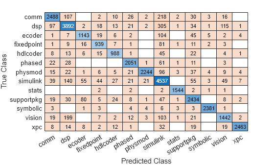
Predict labels for the observations that fitcecoc did not use in training the folds.
label = kfoldPredict(CVMdl);
Because there is one regularization strength in CVMdl, label is a column vector of predictions containing as many rows as observations in X.
Construct a confusion matrix.
cm = confusionchart(Y,label);
Load the NLP data set. Transpose the predictor data.
For simplicity, use the label 'others' for all observations in Y that are not 'simulink', 'dsp', or 'comm'.
Y(~(ismember(Y,{'simulink','dsp','comm'}))) = 'others';
Create a linear classification model template that specifies optimizing the objective function using SpaRSA.
t = templateLinear('Solver','sparsa');
Cross-validate an ECOC model of linear classification models using 5-fold cross-validation. Specify that the predictor observations correspond to columns.
rng(1); % For reproducibility CVMdl = fitcecoc(X,Y,'Learners',t,'KFold',5,'ObservationsIn','columns'); CMdl1 = CVMdl.Trained{1}
CMdl1 = CompactClassificationECOC ResponseName: 'Y' ClassNames: [comm dsp simulink others] ScoreTransform: 'none' BinaryLearners: {6×1 cell} CodingMatrix: [4×6 double]
Properties, Methods
CVMdl is a ClassificationPartitionedLinearECOC model. It contains the property Trained, which is a 5-by-1 cell array holding a CompactClassificationECOC models that the software trained using the training set of each fold.
By default, the linear classification models that compose the ECOC models use SVMs. SVM scores are signed distances from the observation to the decision boundary. Therefore, the domain is (-∞,∞). Create a custom binary loss function that:
- Maps the coding design matrix (M) and positive-class classification scores (s) for each learner to the binary loss for each observation
- Uses linear loss
- Aggregates the binary learner loss using the median.
You can create a separate function for the binary loss function, and then save it on the MATLAB® path. Or, you can specify an anonymous binary loss function.
customBL = @(M,s)median(1 - (M.*s),2,'omitnan')/2;
Predict cross-validation labels and estimate the median binary loss per class. Print the median negative binary losses per class for a random set of 10 out-of-fold observations.
[label,NegLoss] = kfoldPredict(CVMdl,'BinaryLoss',customBL);
idx = randsample(numel(label),10); table(Y(idx),label(idx),NegLoss(idx,1),NegLoss(idx,2),NegLoss(idx,3),... NegLoss(idx,4),'VariableNames',[{'True'};{'Predicted'};... categories(CVMdl.ClassNames)])
ans=10×6 table True Predicted comm dsp simulink others ________ _________ _________ ________ ________ _______
others      others         -1.2319     -1.0488    0.048758     1.6175
simulink    simulink       -16.407     -12.218      21.531     11.218
dsp         dsp            -0.7387    -0.11534    -0.88466    -0.2613
others      others         -0.1251     -0.8749    -0.99766    0.14517
dsp         dsp             2.5867      6.4187     -3.5867    -4.4165
others      others       -0.025358     -1.2287    -0.97464    0.19747
others      others         -2.6725    -0.56708    -0.51092     2.7453
others      others         -1.1605    -0.88321    -0.11679    0.43504
others      others         -1.9511     -1.3175     0.24735    0.95111
simulink    others          -7.848     -5.8203      4.8203     6.8457
The software predicts the label based on the maximum negated loss.
ECOC models composed of linear classification models return posterior probabilities for logistic regression learners only. This example requires the Parallel Computing Toolbox™ and the Optimization Toolbox™
Load the NLP data set and preprocess the data as in Specify Custom Binary Loss.
load nlpdata X = X'; Y(~(ismember(Y,{'simulink','dsp','comm'}))) = 'others';
Create a set of 5 logarithmically-spaced regularization strengths from  through
  .
.
Lambda = logspace(-6,-0.5,5);
Create a linear classification model template that specifies optimizing the objective function using SpaRSA and to use logistic regression learners.
t = templateLinear('Solver','sparsa','Learner','logistic','Lambda',Lambda);
Cross-validate an ECOC model of linear classification models using 5-fold cross-validation. Specify that the predictor observations correspond to columns, and to use parallel computing.
rng(1); % For reproducibility Options = statset('UseParallel',true); CVMdl = fitcecoc(X,Y,'Learners',t,'KFold',5,'ObservationsIn','columns',... 'Options',Options);
Starting parallel pool (parpool) using the 'local' profile ... Connected to the parallel pool (number of workers: 6).
Predict the cross-validated posterior class probabilities. Specify to use parallel computing and to estimate posterior probabilities using quadratic programming.
[label,,,Posterior] = kfoldPredict(CVMdl,'Options',Options,...
'PosteriorMethod','qp');
size(label)
label(3,4)
size(Posterior)
Posterior(3,:,4)
ans =
31572 5ans =
categorical
others ans =
31572 4 5ans =
0.0285 0.0373 0.1714 0.7627Because there are five regularization strengths:
labelis a 31572-by-5 categorical array.label(3,4)is the predicted, cross-validated label for observation 3 using the model trained with regularization strengthLambda(4).Posterioris a 31572-by-4-by-5 matrix.Posterior(3,:,4)is the vector of all estimated, posterior class probabilities for observation 3 using the model trained with regularization strengthLambda(4). The order of the second dimension corresponds toCVMdl.ClassNames. Display a random set of 10 posterior class probabilities.
Display a random sample of cross-validated labels and posterior probabilities for the model trained using Lambda(4).
idx = randsample(size(label,1),10); table(Y(idx),label(idx,4),Posterior(idx,1,4),Posterior(idx,2,4),... Posterior(idx,3,4),Posterior(idx,4,4),... 'VariableNames',[{'True'};{'Predicted'};categories(CVMdl.ClassNames)])
ans =
10×6 table
  True      Predicted       comm          dsp        simulink     others
________    _________    __________    __________    ________    _________

others      others         0.030275      0.022142     0.10416      0.84342
simulink    simulink     3.4954e-05    4.2982e-05     0.99832    0.0016016
dsp         others          0.15787       0.25718     0.18848      0.39647
others      others         0.094177      0.062712     0.12921      0.71391
dsp         dsp           0.0057979       0.89703    0.015098     0.082072
others      others         0.086084      0.054836    0.086165      0.77292
others      others        0.0062338     0.0060492    0.023816       0.9639
others      others          0.06543      0.075097     0.17136      0.68812
others      others         0.051843      0.025566     0.13299       0.7896
simulink    simulink     0.00044059    0.00049753     0.70958      0.28948
More About
The binary loss is a function of the class and classification score that determines how well a binary learner classifies an observation into the class. The decoding scheme of an ECOC model specifies how the software aggregates the binary losses and determines the predicted class for each observation.
Assume the following:
- mkj is element (k,j) of the coding design matrix_M_—that is, the code corresponding to class_k_ of binary learner j.M is a K_-by-B matrix, where K is the number of classes, and_B is the number of binary learners.
- sj is the score of binary learner_j_ for an observation.
- g is the binary loss function.
- k^ is the predicted class for the observation.
The software supports two decoding schemes:
- Loss-based decoding [3] (
Decodingis"lossbased") — The predicted class of an observation corresponds to the class that produces the minimum average of the binary losses over all binary learners. - Loss-weighted decoding [4] (
Decodingis"lossweighted") — The predicted class of an observation corresponds to the class that produces the minimum average of the binary losses over the binary learners for the corresponding class.
The denominator corresponds to the number of binary learners for class_k_. [1] suggests that loss-weighted decoding improves classification accuracy by keeping loss values for all classes in the same dynamic range.
The predict, resubPredict, andkfoldPredict functions return the negated value of the objective function of argmin as the second output argument (NegLoss) for each observation and class.
This table summarizes the supported binary loss functions, where_yj_ is a class label for a particular binary learner (in the set {–1,1,0}), sj is the score for observation j, and_g_(yj,sj) is the binary loss function.
| Value | Description | Score Domain | g(yj,sj) |
|---|---|---|---|
| "binodeviance" | Binomial deviance | (–∞,∞) | log[1 + exp(–2_yjsj_)]/[2log(2)] |
| "exponential" | Exponential | (–∞,∞) | exp(–yjsj)/2 |
| "hamming" | Hamming | [0,1] or (–∞,∞) | [1 – sign(yjsj)]/2 |
| "hinge" | Hinge | (–∞,∞) | max(0,1 – yjsj)/2 |
| "linear" | Linear | (–∞,∞) | (1 – yjsj)/2 |
| "logit" | Logistic | (–∞,∞) | log[1 + exp(–yjsj)]/[2log(2)] |
| "quadratic" | Quadratic | [0,1] | [1 – yj(2_sj_ – 1)]2/2 |
The software normalizes binary losses so that the loss is 0.5 when_yj_ = 0, and aggregates using the average of the binary learners [1].
Do not confuse the binary loss with the overall classification loss (specified by theLossFun name-value argument of the kfoldLoss andkfoldPredict object functions), which measures how well an ECOC classifier performs as a whole.
Algorithms
The software can estimate class posterior probabilities by minimizing the Kullback-Leibler divergence or by using quadratic programming. For the following descriptions of the posterior estimation algorithms, assume that:
- mkj is the element (k,j) of the coding design matrix_M_.
- I is the indicator function.
- p^k is the class posterior probability estimate for class_k_ of an observation, k = 1,...,K.
- rj is the positive-class posterior probability for binary learner j. That is,rj is the probability that binary learner j classifies an observation into the positive class, given the training data.
By default, the software minimizes the Kullback-Leibler divergence to estimate class posterior probabilities. The Kullback-Leibler divergence between the expected and observed positive-class posterior probabilities is
where wj=∑Sjwi∗ is the weight for binary learner j.
- Sj is the set of observation indices on which binary learner j is trained.
- wi∗ is the weight of observation i.
The software minimizes the divergence iteratively. The first step is to choose initial values p^k(0); k=1,...,K for the class posterior probabilities.
- If you do not specify
'NumKLIterations', then the software tries both sets of deterministic initial values described next, and selects the set that minimizes Δ.- p^k(0)=1/K; k=1,...,K.
- p^k(0); k=1,...,K is the solution of the system
where_M_01 is_M_ with all_mkj_ = –1 replaced with 0, and r is a vector of positive-class posterior probabilities returned by the L binary learners [Dietterich et al.]. The software uses lsqnonneg to solve the system.
- If you specify
'NumKLIterations',c, wherecis a natural number, then the software does the following to choose the set p^k(0); k=1,...,K, and selects the set that minimizes Δ.- The software tries both sets of deterministic initial values as described previously.
- The software randomly generates
cvectors of length K using rand, and then normalizes each vector to sum to 1.
At iteration t, the software completes these steps:
- Compute
- Estimate the next class posterior probability using
- Normalize p^k(t+1); k=1,...,K so that they sum to 1.
- Check for convergence.
For more details, see [Hastie et al.] and [Zadrozny].
Posterior probability estimation using quadratic programming requires an Optimization Toolbox license. To estimate posterior probabilities for an observation using this method, the software completes these steps:
- Estimate the positive-class posterior probabilities,rj, for binary learners_j_ = 1,...,L.
- Using the relationship between rj and p^k [Wu et al.], minimize
with respect to p^k and the restrictions
The software performs minimization using quadprog (Optimization Toolbox).
References
[1] Allwein, E., R. Schapire, and Y. Singer. “Reducing multiclass to binary: A unifying approach for margin classifiers.” Journal of Machine Learning Research. Vol. 1, 2000, pp. 113–141.
[2] Dietterich, T., and G. Bakiri. “Solving Multiclass Learning Problems Via Error-Correcting Output Codes.”Journal of Artificial Intelligence Research. Vol. 2, 1995, pp. 263–286.
[3] Escalera, S., O. Pujol, and P. Radeva. “Separability of ternary codes for sparse designs of error-correcting output codes.”Pattern Recog. Lett. Vol. 30, Issue 3, 2009, pp. 285–297.
[4] Escalera, S., O. Pujol, and P. Radeva. “On the decoding process in ternary error-correcting output codes.” IEEE Transactions on Pattern Analysis and Machine Intelligence. Vol. 32, Issue 7, 2010, pp. 120–134.
[5] Hastie, T., and R. Tibshirani. “Classification by Pairwise Coupling.” Annals of Statistics. Vol. 26, Issue 2, 1998, pp. 451–471.
[6] Wu, T. F., C. J. Lin, and R. Weng. “Probability Estimates for Multi-Class Classification by Pairwise Coupling.”Journal of Machine Learning Research. Vol. 5, 2004, pp. 975–1005.
[7] Zadrozny, B. “Reducing Multiclass to Binary by Coupling Probability Estimates.” NIPS 2001: Proceedings of Advances in Neural Information Processing Systems 14, 2001, pp. 1041–1048.
Extended Capabilities
To run in parallel, specify the Options name-value argument in the call to this function and set the UseParallel field of the options structure to true usingstatset:
Options=statset(UseParallel=true)
For more information about parallel computing, see Run MATLAB Functions with Automatic Parallel Support (Parallel Computing Toolbox).
Version History
Introduced in R2016a
Starting in R2023b, the following classification model object functions use observations with missing predictor values as part of resubstitution ("resub") and cross-validation ("kfold") computations for classification edges, losses, margins, and predictions.
In previous releases, the software omitted observations with missing predictor values from the resubstitution and cross-validation computations.