kfoldPredict - Classify observations in cross-validated kernel ECOC model - MATLAB (original) (raw)
Classify observations in cross-validated kernel ECOC model
Syntax
Description
[label](#mw%5Fe9239ee5-9f72-45e2-924e-97f623be087d) = kfoldPredict([CVMdl](#mw%5Fa7c6d187-7086-4884-8102-65cbcf8d26c5%5Fsep%5Fshared-CVMdl)) returns class labels predicted by the cross-validated kernel ECOC model (ClassificationPartitionedKernelECOC) CVMdl. For every fold,kfoldPredict predicts class labels for validation-fold observations using a model trained on training-fold observations. kfoldPredict applies the same data used to create CVMdl (see fitcecoc).
The software predicts the classification of an observation by assigning the observation to the class yielding the largest negated average binary loss (or, equivalently, the smallest average binary loss).
[label](#mw%5Fe9239ee5-9f72-45e2-924e-97f623be087d) = kfoldPredict([CVMdl](#mw%5Fa7c6d187-7086-4884-8102-65cbcf8d26c5%5Fsep%5Fshared-CVMdl),[Name,Value](#namevaluepairarguments)) returns predicted class labels with additional options specified by one or more name-value pair arguments. For example, specify the posterior probability estimation method, decoding scheme, or verbosity level.
[[label](#mw%5Fe9239ee5-9f72-45e2-924e-97f623be087d),[NegLoss](#mw%5F56e1cc78-95ee-4696-91c1-04501e3455cb),[PBScore](#mw%5Fe7e7e5b2-01d1-47fc-aef2-01f6c3833e43)] = kfoldPredict(___) additionally returns negated values of the average binary loss per class (NegLoss) for validation-fold observations and positive-class scores (PBScore) for validation-fold observations classified by each binary learner, using any of the input argument combinations in the previous syntaxes.
If the coding matrix varies across folds (that is, the coding scheme issparserandom or denserandom), thenPBScore is empty ([]).
[[label](#mw%5Fe9239ee5-9f72-45e2-924e-97f623be087d),[NegLoss](#mw%5F56e1cc78-95ee-4696-91c1-04501e3455cb),[PBScore](#mw%5Fe7e7e5b2-01d1-47fc-aef2-01f6c3833e43),[Posterior](#mw%5F27dbe2bf-d045-4708-b85d-d70abcd8ef38)] = kfoldPredict(___) additionally returns posterior class probability estimates for validation-fold observations (Posterior).
To obtain posterior class probabilities, the kernel classification binary learners must be logistic regression models. Otherwise, kfoldPredict throws an error.
Examples
Classify observations using a cross-validated, multiclass kernel ECOC classifier, and display the confusion matrix for the resulting classification.
Load Fisher's iris data set. X contains flower measurements, and Y contains the names of flower species.
load fisheriris X = meas; Y = species;
Cross-validate an ECOC model composed of kernel binary learners.
rng(1); % For reproducibility CVMdl = fitcecoc(X,Y,'Learners','kernel','CrossVal','on')
CVMdl = ClassificationPartitionedKernelECOC CrossValidatedModel: 'KernelECOC' ResponseName: 'Y' NumObservations: 150 KFold: 10 Partition: [1×1 cvpartition] ClassNames: {'setosa' 'versicolor' 'virginica'} ScoreTransform: 'none'
Properties, Methods
CVMdl is a ClassificationPartitionedKernelECOC model. By default, the software implements 10-fold cross-validation. To specify a different number of folds, use the 'KFold' name-value pair argument instead of 'Crossval'.
Classify the observations that fitcecoc does not use in training the folds.
label = kfoldPredict(CVMdl);
Construct a confusion matrix to compare the true classes of the observations to their predicted labels.
C = confusionchart(Y,label);
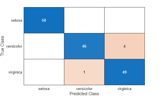
The CVMdl model misclassifies four 'versicolor' irises as 'virginica' irises and misclassifies one 'virginica' iris as a 'versicolor' iris.
Load Fisher's iris data set. X contains flower measurements, and Y contains the names of flower species.
load fisheriris X = meas; Y = species;
Cross-validate an ECOC model of kernel classification models using 5-fold cross-validation.
rng(1); % For reproducibility CVMdl = fitcecoc(X,Y,'Learners','kernel','KFold',5)
CVMdl = ClassificationPartitionedKernelECOC CrossValidatedModel: 'KernelECOC' ResponseName: 'Y' NumObservations: 150 KFold: 5 Partition: [1×1 cvpartition] ClassNames: {'setosa' 'versicolor' 'virginica'} ScoreTransform: 'none'
Properties, Methods
CVMdl is a ClassificationPartitionedKernelECOC model. It contains the property Trained, which is a 5-by-1 cell array of CompactClassificationECOC models.
By default, the kernel classification models that compose the CompactClassificationECOC models use SVMs. SVM scores are signed distances from the observation to the decision boundary. Therefore, the domain is (-∞,∞). Create a custom binary loss function that:
- Maps the coding design matrix (M) and positive-class classification scores (s) for each learner to the binary loss for each observation
- Uses linear loss
- Aggregates the binary learner loss using the median
You can create a separate function for the binary loss function, and then save it on the MATLAB® path. Or, you can specify an anonymous binary loss function. In this case, create a function handle (customBL) to an anonymous binary loss function.
customBL = @(M,s)median(1 - (M.*s),2,'omitnan')/2;
Predict cross-validation labels and estimate the median binary loss per class. Print the median negative binary losses per class for a random set of 10 observations.
[label,NegLoss] = kfoldPredict(CVMdl,'BinaryLoss',customBL);
idx = randsample(numel(label),10); table(Y(idx),label(idx),NegLoss(idx,1),NegLoss(idx,2),NegLoss(idx,3),... 'VariableNames',[{'True'};{'Predicted'};... unique(CVMdl.ClassNames)])
ans=10×5 table True Predicted setosa versicolor virginica ______________ ______________ ________ __________ _________
{'setosa'    }    {'setosa'    }     0.20926     -0.84572     -0.86354
{'setosa'    }    {'setosa'    }     0.16144     -0.90572     -0.75572
{'virginica' }    {'versicolor'}    -0.83532     -0.12157     -0.54311
{'virginica' }    {'virginica' }    -0.97235     -0.69759      0.16994
{'virginica' }    {'virginica' }    -0.89441     -0.69937     0.093778
{'virginica' }    {'virginica' }    -0.86774     -0.47297     -0.15929
{'setosa'    }    {'setosa'    }     -0.1026     -0.69671     -0.70069
{'setosa'    }    {'setosa'    }      0.1001     -0.89163     -0.70848
{'virginica' }    {'virginica' }     -1.0106     -0.52919     0.039829
{'versicolor'}    {'versicolor'}     -1.0298     0.027354     -0.49757
The cross-validated model correctly predicts the labels for 9 of the 10 random observations.
Estimate posterior class probabilities using a cross-validated, multiclass kernel ECOC classification model. Kernel classification models return posterior probabilities for logistic regression learners only.
Load Fisher's iris data set. X contains flower measurements, and Y contains the names of flower species.
load fisheriris X = meas; Y = species;
Create a kernel template for the binary kernel classification models. Specify to fit logistic regression learners.
t = templateKernel('Learner','logistic')
t = Fit template for classification Kernel.
         BetaTolerance: []
             BlockSize: []
         BoxConstraint: []
               Epsilon: []
NumExpansionDimensions: []
     GradientTolerance: []
    HessianHistorySize: []
        IterationLimit: []
           KernelScale: []
                Lambda: []
               Learner: 'logistic'
          LossFunction: []
                Stream: []
        VerbosityLevel: []
       StandardizeData: []
               Version: 1
                Method: 'Kernel'
                  Type: 'classification'
t is a kernel template. Most of its properties are empty. When training an ECOC classifier using the template, the software sets the applicable properties to their default values.
Cross-validate an ECOC model using the kernel template.
rng('default'); % For reproducibility CVMdl = fitcecoc(X,Y,'Learners',t,'CrossVal','on')
CVMdl = ClassificationPartitionedKernelECOC CrossValidatedModel: 'KernelECOC' ResponseName: 'Y' NumObservations: 150 KFold: 10 Partition: [1×1 cvpartition] ClassNames: {'setosa' 'versicolor' 'virginica'} ScoreTransform: 'none'
Properties, Methods
CVMdl is a ClassificationPartitionedECOC model. By default, the software uses 10-fold cross-validation.
Predict the validation-fold class posterior probabilities.
[label,,,Posterior] = kfoldPredict(CVMdl);
The software assigns an observation to the class that yields the smallest average binary loss. Because all binary learners are computing posterior probabilities, the binary loss function is quadratic.
Display the posterior probabilities for 10 randomly selected observations.
idx = randsample(size(X,1),10); CVMdl.ClassNames
ans = 3×1 cell {'setosa' } {'versicolor'} {'virginica' }
table(Y(idx),label(idx),Posterior(idx,:),... 'VariableNames',{'TrueLabel','PredLabel','Posterior'})
ans=10×3 table
TrueLabel PredLabel Posterior
______________ ______________ ________________________________
{'setosa'    }    {'setosa'    }     0.68216     0.18546     0.13238
{'virginica' }    {'virginica' }      0.1581     0.14405     0.69785
{'virginica' }    {'virginica' }    0.071807    0.093291      0.8349
{'setosa'    }    {'setosa'    }     0.74918     0.11434     0.13648
{'versicolor'}    {'versicolor'}     0.09375     0.67149     0.23476
{'versicolor'}    {'versicolor'}    0.036202     0.85544     0.10836
{'versicolor'}    {'versicolor'}      0.2252     0.50473     0.27007
{'virginica' }    {'virginica' }    0.061562     0.11086     0.82758
{'setosa'    }    {'setosa'    }     0.42448     0.21181     0.36371
{'virginica' }    {'virginica' }    0.082705      0.1428      0.7745
The columns of Posterior correspond to the class order of CVMdl.ClassNames.
Input Arguments
Name-Value Arguments
Specify optional pairs of arguments asName1=Value1,...,NameN=ValueN, where Name is the argument name and Value is the corresponding value. Name-value arguments must appear after other arguments, but the order of the pairs does not matter.
Before R2021a, use commas to separate each name and value, and enclose Name in quotes.
Example: kfoldPredict(CVMdl,'PosteriorMethod','qp') specifies to estimate multiclass posterior probabilities by solving a least-squares problem using quadratic programming.
Data Types: char | string | function_handle
Decoding scheme that aggregates the binary losses, specified as the comma-separated pair consisting of 'Decoding' and'lossweighted' or 'lossbased'. For more information, see Binary Loss.
Example: 'Decoding','lossbased'
Number of random initial values for fitting posterior probabilities by Kullback-Leibler divergence minimization, specified as the comma-separated pair consisting of 'NumKLInitializations' and a nonnegative integer scalar.
If you do not request the fourth output argument (Posterior) and set 'PosteriorMethod','kl' (the default), then the software ignores the value of NumKLInitializations.
For more details, see Posterior Estimation Using Kullback-Leibler Divergence.
Example: 'NumKLInitializations',5
Data Types: single | double
Posterior probability estimation method, specified as the comma-separated pair consisting of 'PosteriorMethod' and 'kl' or'qp'.
- If
PosteriorMethodis'kl', then the software estimates multiclass posterior probabilities by minimizing the Kullback-Leibler divergence between the predicted and expected posterior probabilities returned by binary learners. For details, see Posterior Estimation Using Kullback-Leibler Divergence. - If
PosteriorMethodis'qp', then the software estimates multiclass posterior probabilities by solving a least-squares problem using quadratic programming. You need an Optimization Toolbox™ license to use this option. For details, see Posterior Estimation Using Quadratic Programming. - If you do not request the fourth output argument (Posterior), then the software ignores the value of
PosteriorMethod.
Example: 'PosteriorMethod','qp'
Data Types: single | double
Output Arguments
Predicted class labels, returned as a categorical or character array, logical or numeric vector, or cell array of character vectors.
label has the same data type and number of rows asCVMdl.Y.
The software predicts the classification of an observation by assigning the observation to the class yielding the largest negated average binary loss (or, equivalently, the smallest average binary loss).
Negated average binary losses, returned as a numeric matrix.NegLoss is an _n_-by-K matrix, where n is the number of observations (size(CVMdl.Y,1)) and K is the number of unique classes (size(CVMdl.ClassNames,1)).
NegLoss(i,k) is the negated average binary loss for classifying observation_i_ into the _k_th class.
- If Decoding is
'lossbased', thenNegLoss(i,k)is the negated sum of the binary losses divided by the total number of binary learners. - If
Decodingis'lossweighted', thenNegLoss(i,k)is the negated sum of the binary losses divided by the number of binary learners for the _k_th class.
For more details, see Binary Loss.
Positive-class scores for each binary learner, returned as a numeric matrix.PBScore is an _n_-by-B matrix, where n is the number of observations (size(CVMdl.Y,1)) and B is the number of binary learners (size(CVMdl.CodingMatrix,2)).
If the coding matrix varies across folds (that is, the coding scheme issparserandom or denserandom), thenPBScore is empty ([]).
Posterior class probabilities, returned as a numeric matrix.Posterior is an _n_-by-K matrix, where n is the number of observations (size(CVMdl.Y,1)) and K is the number of unique classes (size(CVMdl.ClassNames,1)).
To return posterior probabilities, each kernel classification binary learner must have its Learner property set to 'logistic'. Otherwise, the software throws an error.
More About
The binary loss is a function of the class and classification score that determines how well a binary learner classifies an observation into the class. The decoding scheme of an ECOC model specifies how the software aggregates the binary losses and determines the predicted class for each observation.
Assume the following:
- mkj is element (k,j) of the coding design matrix_M_—that is, the code corresponding to class_k_ of binary learner j.M is a K_-by-B matrix, where K is the number of classes, and_B is the number of binary learners.
- sj is the score of binary learner_j_ for an observation.
- g is the binary loss function.
- k^ is the predicted class for the observation.
The software supports two decoding schemes:
- Loss-based decoding [3] (
Decodingis"lossbased") — The predicted class of an observation corresponds to the class that produces the minimum average of the binary losses over all binary learners. - Loss-weighted decoding [4] (
Decodingis"lossweighted") — The predicted class of an observation corresponds to the class that produces the minimum average of the binary losses over the binary learners for the corresponding class.
The denominator corresponds to the number of binary learners for class_k_. [1] suggests that loss-weighted decoding improves classification accuracy by keeping loss values for all classes in the same dynamic range.
The predict, resubPredict, andkfoldPredict functions return the negated value of the objective function of argmin as the second output argument (NegLoss) for each observation and class.
This table summarizes the supported binary loss functions, where_yj_ is a class label for a particular binary learner (in the set {–1,1,0}), sj is the score for observation j, and_g_(yj,sj) is the binary loss function.
| Value | Description | Score Domain | g(yj,sj) |
|---|---|---|---|
| "binodeviance" | Binomial deviance | (–∞,∞) | log[1 + exp(–2_yjsj_)]/[2log(2)] |
| "exponential" | Exponential | (–∞,∞) | exp(–yjsj)/2 |
| "hamming" | Hamming | [0,1] or (–∞,∞) | [1 – sign(yjsj)]/2 |
| "hinge" | Hinge | (–∞,∞) | max(0,1 – yjsj)/2 |
| "linear" | Linear | (–∞,∞) | (1 – yjsj)/2 |
| "logit" | Logistic | (–∞,∞) | log[1 + exp(–yjsj)]/[2log(2)] |
| "quadratic" | Quadratic | [0,1] | [1 – yj(2_sj_ – 1)]2/2 |
The software normalizes binary losses so that the loss is 0.5 when_yj_ = 0, and aggregates using the average of the binary learners [1].
Do not confuse the binary loss with the overall classification loss (specified by theLossFun name-value argument of the kfoldLoss andkfoldPredict object functions), which measures how well an ECOC classifier performs as a whole.
Algorithms
The software can estimate class posterior probabilities by minimizing the Kullback-Leibler divergence or by using quadratic programming. For the following descriptions of the posterior estimation algorithms, assume that:
- mkj is the element (k,j) of the coding design matrix_M_.
- I is the indicator function.
- p^k is the class posterior probability estimate for class_k_ of an observation, k = 1,...,K.
- rj is the positive-class posterior probability for binary learner j. That is,rj is the probability that binary learner j classifies an observation into the positive class, given the training data.
By default, the software minimizes the Kullback-Leibler divergence to estimate class posterior probabilities. The Kullback-Leibler divergence between the expected and observed positive-class posterior probabilities is
where wj=∑Sjwi∗ is the weight for binary learner j.
- Sj is the set of observation indices on which binary learner j is trained.
- wi∗ is the weight of observation i.
The software minimizes the divergence iteratively. The first step is to choose initial values p^k(0); k=1,...,K for the class posterior probabilities.
- If you do not specify
'NumKLIterations', then the software tries both sets of deterministic initial values described next, and selects the set that minimizes Δ.- p^k(0)=1/K; k=1,...,K.
- p^k(0); k=1,...,K is the solution of the system
where_M_01 is_M_ with all_mkj_ = –1 replaced with 0, and r is a vector of positive-class posterior probabilities returned by the L binary learners [Dietterich et al.]. The software uses lsqnonneg to solve the system.
- If you specify
'NumKLIterations',c, wherecis a natural number, then the software does the following to choose the set p^k(0); k=1,...,K, and selects the set that minimizes Δ.- The software tries both sets of deterministic initial values as described previously.
- The software randomly generates
cvectors of length K using rand, and then normalizes each vector to sum to 1.
At iteration t, the software completes these steps:
- Compute
- Estimate the next class posterior probability using
- Normalize p^k(t+1); k=1,...,K so that they sum to 1.
- Check for convergence.
For more details, see [Hastie et al.] and [Zadrozny].
Posterior probability estimation using quadratic programming requires an Optimization Toolbox license. To estimate posterior probabilities for an observation using this method, the software completes these steps:
- Estimate the positive-class posterior probabilities,rj, for binary learners_j_ = 1,...,L.
- Using the relationship between rj and p^k [Wu et al.], minimize
with respect to p^k and the restrictions
The software performs minimization using quadprog (Optimization Toolbox).
References
[1] Allwein, E., R. Schapire, and Y. Singer. “Reducing multiclass to binary: A unifying approach for margin classifiers.” Journal of Machine Learning Research. Vol. 1, 2000, pp. 113–141.
[2] Dietterich, T., and G. Bakiri. “Solving Multiclass Learning Problems Via Error-Correcting Output Codes.” Journal of Artificial Intelligence Research. Vol. 2, 1995, pp. 263–286.
[3] Escalera, S., O. Pujol, and P. Radeva. “Separability of ternary codes for sparse designs of error-correcting output codes.”Pattern Recog. Lett. Vol. 30, Issue 3, 2009, pp. 285–297.
[4] Escalera, S., O. Pujol, and P. Radeva. “On the decoding process in ternary error-correcting output codes.” IEEE Transactions on Pattern Analysis and Machine Intelligence. Vol. 32, Issue 7, 2010, pp. 120–134.
[5] Hastie, T., and R. Tibshirani. “Classification by Pairwise Coupling.” Annals of Statistics. Vol. 26, Issue 2, 1998, pp. 451–471.
[6] Wu, T. F., C. J. Lin, and R. Weng. “Probability Estimates for Multi-Class Classification by Pairwise Coupling.” Journal of Machine Learning Research. Vol. 5, 2004, pp. 975–1005.
[7] Zadrozny, B. “Reducing Multiclass to Binary by Coupling Probability Estimates.” NIPS 2001: Proceedings of Advances in Neural Information Processing Systems 14, 2001, pp. 1041–1048.
Extended Capabilities
To run in parallel, specify the Options name-value argument in the call to this function and set the UseParallel field of the options structure to true usingstatset:
Options=statset(UseParallel=true)
For more information about parallel computing, see Run MATLAB Functions with Automatic Parallel Support (Parallel Computing Toolbox).
Version History
Introduced in R2018b
Starting in R2023b, the following classification model object functions use observations with missing predictor values as part of resubstitution ("resub") and cross-validation ("kfold") computations for classification edges, losses, margins, and predictions.
In previous releases, the software omitted observations with missing predictor values from the resubstitution and cross-validation computations.