Statistics For Data Science (original) (raw)
Last Updated : 15 Apr, 2026
Statistics is the science of collecting, analyzing, and interpreting data to uncover patterns and make decisions. In data science, it acts as the backbone for understanding data and building reliable models.
- Summarizes data using measures like mean, median, and variance
- Models uncertainty with probability and distributions
- Tests hypotheses (e.g., A/B testing)
- Finds relationships through regression and correlation
Types of Statistics
There are commonly two types of statistics, which are discussed below:
- **Descriptive Statistics: Descriptive Statistics helps us simplify and organize big chunks of data. This makes large amounts of data easier to understand.
- **Inferential Statistics: Inferential Statistics is a little different. It uses smaller data to conclude a larger group. It helps us predict and draw conclusions about a population.
What is Data in Statistics?
Data is a collection of observations, it can be in the form of numbers, words, measurements, or statements.
Types of Data
**1. **Qualitative Data: This data is descriptive. For example - She is beautiful, He is tall, etc.
**2. Quantitative Data: This is numerical information. For example - A horse has four legs.
- **Discrete Data: It has a particular fixed value and can be counted.
- **Continuous Data: It is not fixed but has a range of data and can be measured.
Basics of Statistics
Basic formulas of statistics are,
| Parameters | Definition | Formulas |
|---|---|---|
| **Population Mean (μ) | Average of the entire group. | \Sigma{\frac{x}{N}} |
| **Sample Mean | Average of a subset of the population | \Sigma{\frac{x}{n}} |
| **Sample/Population Standard Deviation | Measures how spread out the data is from the mean | \text{Population σ} = \sqrt{\frac{1}{N} \sum_{i=1}^{n} (x_i - \mu)^2}\\\\\text{Sample s} = \sqrt{\frac{1}{N-1} \sum_{i=1}^{n} (x_i - \bar{x})^2} |
| **Sample/Population Variance | Shows how far values are from the mean, squared | Variance(Population)~=~\frac{{\sum(x-\overline{x})^2}}{n}\\Variance(Sample)~=~\frac{{\sum(x-\overline{x})^2}}{n-1} |
| **Class Interval(CI) | Range of values in a group | CI = Upper Limit − Lower Limit |
| **Frequency(f) | How often a value appears | Count of occurrences |
| **Range (R) | Difference between largest and smallest values | Range = Max−Min |
Measure of Central Tendency
**1. Mean: The mean can be calculated by summing all values present in the sample divided by total number of values present in the sample or population.
Formula:Mean (\mu) = \frac{Sum \, of \, Values}{Number \, of \, Values}
**2. Median: The median is the middle of a dataset when arranged from lowest to highest or highest to lowest in order to find the median, the data must be sorted. For an odd number of data points the median is the middle value and for an even number of data points median is the average of the two middle values.
**3. Mode: The most frequently occurring value in the Sample or Population is called as Mode.
Measure of Dispersion
- **Range: Range is the difference between the maximum and minimum values of the Sample.
- **Variance (σ²): Variance is a measure of how spread-out values from the mean by measuring the dispersion around the Mean.
Formula:\sigma^2~=~\frac{\Sigma(X-\mu)^2}{n}
- **Standard Deviation (σ): Standard Deviation is the square root of variance. The measuring unit of S.D. is same as the Sample values' unit. It indicates the average distance of data points from the mean and is widely used due to its intuitive interpretation.
Formula:\sigma=\sqrt(\sigma^2)=\sqrt(\frac{\Sigma(X-\mu)^2}{n})
- **Interquartile Range (IQR): The range between the first quartile (Q1) and the third quartile (Q3). It is less sensitive to extreme values than the range. To compute IQR, calculate the values of the first and third quartile by arranging the data in ascending order. Then, calculate the mean of each half of the dataset.
Formula: IQR = Q_3 -Q_1
- **Quartiles: Quartiles divides the dataset into four equal parts:
Q1 (First Quartile): Median of the lower 50% of the dataset (25th percentile).
Q2 (Second Quartile / Median): Median of the entire dataset (50th percentile).
Q3 (Third Quartile): Median of the upper 50% of the dataset (75th percentile).
- **Mean Absolute Deviation: The average of the absolute differences between each data point and the mean. It provides a measure of the average deviation from the mean.
Formula: Mean \, Absolute \, Deviation = \frac{\sum_{i=1}^{n}{|X - \mu|}}{n}
- **Coefficient of Variation (CV):
CV is the ratio of the standard deviation to the mean, expressed as a percentage. It is useful for comparing the relative variability of different datasets.
CV = (\frac{\sigma}{\mu}) * 100
Measure of Shape
1. Skewness
Skewness is the measure of asymmetry of probability distribution about its mean.
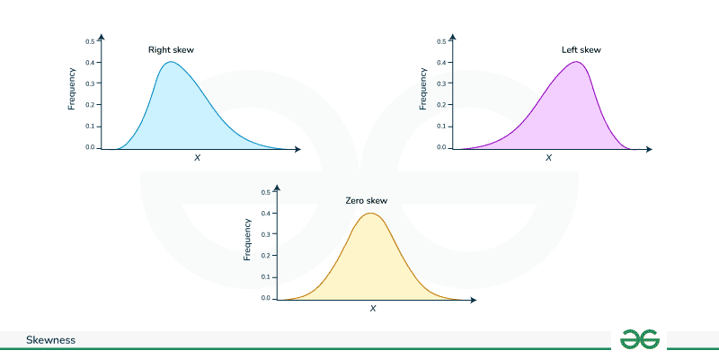
Types of Skewed data
**Types of Skewed data
- **Positive Skew (Right): Mean > Median
- **Negative Skew (Left): Mean < Median
- **Symmetrical: Mean = Median
2. Kurtosis
Kurtosis quantifies the degree to which a probability distribution deviates from the normal distribution. It assesses the "tailedness" of the distribution, indicating whether it has heavier or lighter tails than a normal distribution. High kurtosis implies more extreme values in the distribution, while low kurtosis indicates a flatter distribution.

Types of Kurtosis
Types of Kurtosis
- **Mesokurtic: Normal distribution (kurtosis = 3)
- **Leptokurtic: Heavy tails (kurtosis > 3)
- **Platykurtic: Light tails (kurtosis < 3)
Measure of Relationship
- **Covariance: Covariance measures the degree to which two variables change together.
Cov(x,y) = \frac{\sum(X_i-\overline{X})(Y_i - \overline{Y})}{n}
- **Correlation: Correlation measures the strength and direction of the linear relationship between two variables. It is represented by correlation coefficient which ranges from -1 to 1. A positive correlation indicates a direct relationship, while a negative correlation implies an inverse relationship. Pearson's correlation coefficient is given by:
\rho(X, Y) = \frac{cov(X,Y)}{\sigma_X \sigma_Y}
Probability Theory
Here are some basic concepts or terminologies used in probability:
| Term | Definition |
|---|---|
| Sample Space | The set of all possible outcomes in a probability experiment. |
| Event | A subset of the sample space. |
| Joint Probability (Intersection of Event) | Probability of occurring events A and B. Formula: P(A and B) = P(A) × P(B) |
| Union of Events | Probability of occurring events A or B. Formula: P(A or B) = P(A) + P(B) - P(A and B) |
| Conditional Probability | Probability of occurring events A when event B has occurred. Formula: P(A | B) = P(A and B)/P(B) |
Bayes Theorem
Bayes' Theorem is a fundamental concept in probability theory that relates conditional probabilities. It is named after the Reverend Thomas Bayes, who first introduced the theorem. Bayes' Theorem is a mathematical formula that provides a way to update probabilities based on new evidence. The formula is as follows:
P(A|B) = \frac{P(B|A) \times P(A)}{P(B)}
where
- _P(_A_∣__B): Probability of event A given that event B has occurred (posterior probability).
- _P(_B_∣__A): Probability of event B given that event A has occurred (likelihood).
Types of Probability Functions
- **Probability Mass Function(PMF): Probability Mass Function is a concept of a discrete random variable.
- **Probability Density Function (PDF): Probability Density Function describes the likelihood of a continuous random variable falling within a particular range.
- **Cumulative Distribution Function (CDF): Cumulative Distribution Function gives the probability that a random variable will take a value less than or equal to a given value.
- **Empirical Distribution Function (EDF): Estimates the CDF using observed sample data.
Probability Distributions Functions
1. Normal or Gaussian Distribution
The normal distribution is a continuous probability distribution characterized by its bell-shaped curve and can be by described by mean (μ) and standard deviation (σ).
**Formula: f(X|\mu,\sigma)=\frac{\epsilon^{-0.5(\frac{X-\mu}{\sigma})^2}}{\sigma\sqrt(2\pi)}
**Empirical Rule (68-95-99.7 Rule): ~68% data within 1σ, ~95% within 2σ, ~99.7% within 3σ.

**Use: Detecting outliers, modeling natural phenomena.
**Central Limit Theorem: The Central Limit Theorem (CLT) states that, regardless of the shape of the original population distribution, the sampling distribution of the sample mean will be approximately normally distributed if the sample size tends to infinity.
2. Student t-distribution
The t-distribution, also known as Student's t-distribution, is a probability distribution that is used in statistics.
f(t) =\frac{\Gamma\left(\frac{df+1}{2}\right)}{\sqrt{df\pi} \, \Gamma\left(\frac{df}{2}\right)} \left(1 + \frac{t^2}{df}\right)^{-\frac{df+1}{2}}
- **Parameter: Degrees of freedom (df).
- **Use: Hypothesis testing with small samples.
3. Chi-square Distribution
The chi-squared distribution, denoted as \chi ^2 is a probability distribution used in statistics it is related to the sum of squared standard normal deviates.
\chi^2 = \frac 1{2^{k/2}\Gamma {(k/2)}} x^{{\frac k 2}-1} e^{\frac {-x}2}
4. Binomial Distribution
The binomial distribution models the number of successes in a fixed number of independent Bernoulli trials, where each trial has the same probability of success (_p).
**Formula: P(X=k)=(^n_k)p^k(1-p)^{n-k}
5. Poisson Distribution
The poisson distribution models the number of events that occur in a fixed interval of time or space. It's characterized by a single parameter (_λ), the average rate of occurrence.
**Formula: P(X=k)=\frac{\epsilon^{-\lambda}\lambda^k}{k!}
6. Uniform Distribution
The uniform distribution represents a constant probability for all outcomes in a given range.
Formula: f(X)=\frac{1}{b-a}
Parameter estimation for Statistical Inference
- **Population: Population is entire group about which conclusions are drawn.
- **Sample: Sample is a subset of the population used to make inferences.
- **Expectation (E[x]): Expectation is average or expected value of a random variable.
- **Parameter: A numerical value that describes a population (e.g., μ, σ, p).
- **Statistic: A value computed from sample data to estimate a population parameter.
- **Estimation: The process of inferring population parameters from sample statistics.
- **Estimator: A rule or formula to estimate an unknown parameter.
- **Bias: The difference between an estimator’s expected value and the true parameter.
Bias(\widehat{\theta}) = E(\widehat{\theta}) - \theta
Hypothesis Testing
Hypothesis testing makes inferences about a population parameter based on sample statistic.

**1. Null Hypothesis (H₀): There is no significant difference or effect.
**2. Alternative Hypothesis (H₁): There is a significant effect i.e the given statement can be false.
**3. Degrees of freedom: Degrees of freedom (df) in statistics represent the number of values or quantities in the final calculation of a statistic that are free to vary. It is mainly defined as sample size-one (n-1).
*4. Level of Significance(\alpha)*: This is the threshold used to determine statistical significance. Common values are 0.05, 0.01, or 0.10.
**5. p-value: The p-value probability of observing results if H₀ is true.
- If p ≤ α: reject H₀
- If p > α: fail to reject H₀
**6. Type I Error and Type II Error
- Type I Error that occurs when the null hypothesis is true, but the statistical test incorrectly rejects it. It is often referred to as a "false positive" or "alpha error."
- Type II Error that occurs when the null hypothesis is false, but the statistical test fails to reject it. It is often referred to as a "false negative."
**7. Confidence Intervals: A confidence interval is a range of values that is used to estimate the true value of a population parameter with a certain level of confidence. It provides a measure of the uncertainty or margin of error associated with a sample statistic, such as the sample mean or proportion.
**Example of Hypothesis Testing (Website Redesign)
An e-commerce company wants to know if a website redesign affects average user session time.
- **Before: Mean = 3.5 min, SD = 1.2, n = 50
- **After: Mean = 4.2 min, SD = 1.5, n = 60
**Hypotheses:
- H₀: No change (μ_after − μ_before = 0)
- H₁: Positive change (μ_after − μ_before > 0)
**Significance Level: α = 0.05
**Test: Difference in means -> calculate p-value**Interpretation:
- If p < 0.05: Redesign significantly increased session time
- If p ≥ 0.05: No significant effect
Statistical Tests
Parametric test are statistical methods that make assumption that the data follows normal distribution.
| Z-test | t-test | F-test |
|---|---|---|
| Tests if a sample mean differs from a known population mean. | Compares means when population standard deviation is unknown. | Compares variances of two or more groups. |
| Population standard deviation is known and sample size is large. | Small samples or unknown population standard deviation. | To test if group variances are significantly different. |
| One-Sample Test:Z = \frac{\overline{X}-\mu}{\frac{\sigma}{\sqrt{n}}}Two-Sample Test:Z = \frac{\overline{X_1} -\overline{X_2}}{\sqrt{\frac{\sigma_{1}^{2}}{n_1} + \frac{\sigma_{2}^{2}}{n_2}}} | One- sample: t = \frac{\overline{X}- \mu}{\frac{s}{\sqrt{n}}}Two-Sample Test: t= \frac{\overline{X_1} - \overline{X_2}}{\sqrt{\frac{s_{1}^{2}}{n_1} + \frac{s_{2}^{2}}{n_2}}}Paired t-Test:t=\frac{\overline{d}}{\frac{s_d}{\sqrt{n}}}d= difference | F = \frac{s_{1}^{2}}{s_{2}^{2}} |
ANOVA (Analysis Of Variance)
| Source of Variation | Sum of Squares | Degrees Of Freedom | Mean Squares | F-Value |
|---|---|---|---|---|
| Between Groups | SSB= \Sigma n _1(\bar x_1 - \bar x)^2 | df1=k-1 | MSB= SSB/ (k-1) | f=MSB/MSE |
| Error | SSE=\Sigma\Sigma (\bar x_1 - \bar x)^2 | df2=N-1 | MSE=SSE/(N-k) | |
| Total | SST= SSB+SSE | df3=N-1 |
There are mainly **two types of ANOVA:
1. One-way ANOVA: Compares means of 3+ groups.
- **H₀: All group means are equal
- **H₁: At least one group differs
2. Two-way ANOVA: Tests impact of two categorical variables and their interaction
Chi-Squared Test
The chi-squared test is a statistical test used to determine if there is a significant association between two categorical variables. It compares the observed frequencies in a contingency table with the frequencies.
****Formula:**X^2=\Sigma{\frac{(O_{ij}-E_{ij})^2}{E_{ij}}}
This test is also performed on big data with multiple number of observations.
Non-Parametric Test
Non-parametric test does not make assumptions about the distribution of the data. They are useful when data does not meet the assumptions required for parametric tests.
- **Mann-Whitney U Test: Mann-Whitney U Test is used to determine whether there is a difference between two independent groups when the dependent variable is ordinal or continuous. Applicable when assumptions for a t-test are not met. In it we rank all data points, combines the ranks and calculates the test statistic.
- **Kruskal-Wallis Test: Kruskal-Wallis Test is used to determine whether there are differences among three or more independent groups when the dependent variable is ordinal or continuous. Non-parametric alternative to one-way ANOVA.
A/B Testing or Split Testing
A/B testing, also known as split testing, is a method used to compare two versions (A and B) of a webpage, app, or marketing asset to determine which one performs better.
**Example: a product manager change a website's "Shop Now" button color from green to blue to improve the click-through rate (CTR). Formulating null and alternative hypotheses, users are divided into A and B groups and CTRs are recorded. Statistical tests like chi-square or t-test are applied with a 5% confidence interval. If the p-value is below 5%, the manager may conclude that changing the button color significantly affects CTR, informing decisions for permanent implementation.
Regression
Regression is a statistical technique used to model the relationship between a dependent variable and one or more independent variables.
The equation for regression: y=\alpha+ \beta x
Where,
- _y is the dependent variable,
- _x is the independent variable
- \alpha is the intercept
- \beta is the regression coefficient.
Regression coefficient is a measure of the strength and direction of the relationship between a predictor variable (independent variable) and the response variable (dependent variable) \beta = \frac{\sum(X_i-\overline{X})(Y_i - \overline{Y})}{\sum(X_i-\overline{X})^2}