Last Minute Notes Engineering Mathematics (original) (raw)
Last Updated : 20 Feb, 2026
GATE CSE is a national-level engineering entrance exam in India specifically for Computer Science and Engineering. It's conducted by top Indian institutions like IISc Bangalore and various IITs. In GATE CSE, engineering mathematics is a significant portion of the exam, typically constituting 15% of the total marks. Key topics in engineering mathematics tested in the exam include:
Check Complete **Last Minute Notes for GATE CSE.
Linear Algebra
Matrices
- A matrix is a rectangular array of numbers arranged in rows and columns.
- **Order: Denoted as m × n, where m is the number of rows and n is the number of columns.

This Matrix [M] has 3 rows and 2 columns i.e., order of 3 × 2. Each element of matrix [M] can be referred to by its row and column number. For example, a32 = 0.
**Types of Matrices
- **Square Matrix: m = n.
- **Diagonal Matrix: All non-diagonal elements are zero.
- **Identity Matrix (I): A diagonal matrix with all diagonal elements as 1.
- **Zero Matrix: All elements are zero.
- **Symmetric Matrix: A = AT (Transpose equals the original matrix).
- **Skew-Symmetric Matrix: A = − AT.
- **Orthogonal Matrix: AT A = I, where AT is the transpose.
- **Singular Matrix: Determinant is 0 (det(A) = 0).
- **Non-Singular Matrix: Determinant is non-zero (det(A) ≠ 0).
- **Idempotent Matrix****:** A matrix is said to be idempotent if A2 = A
- **Involutory Matrix****:** A matrix is said to be Involutory if A2 = I.
- **Nilpotent Matrix****:** A square matrix of order n is said to be nilpotent if Ak = 0, k ≤ n.
**Operations on Matrices
Matrix Operations are basic calculations performed on matrices to solve problems or manipulate their structure.
**Transpose of a Matrix: The transpose [M]T of an m x n matrix [M] is the n × m matrix obtained by interchanging the rows and columns of [M]. if A= [aij] m × n , then AT = [bij] n × m where bij = aji
**Properties of transpose of a Matrix:
- (AT)T = A
- (kA)T = k(AT)
- (A ± B)T = AT ± BT
- (AB)T = BT · AT
- (A-1)T = (AT)-1
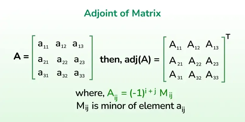
**Adjoint of a Matrix: The adjoint of a square matrix is the transpose of its cofactor matrix.
Read More about **Minor and Cofactors.
**Properties of Adjoint
Some important properties of adjoint include:
- A(Adj A) = (Adj A) A = |A| In
- Adj(AB) = (Adj B) · (Adj A)
- |Adj A|= |A|n-1
- adj(adj(A)) = |A|n-2 · A
- adj(AT) = (adj(A))T
- Adj(kA) = kn-1 Adj(A)
**Inverse of a Matrix
For any square matrix A,
A^{-1} = \frac{Adj A}{|A|}
Here |A| should not be equal to zero, means matrix A should be non-singular.
**Properties of Inverse
- A-1 · A = I
- (A-1)-1 = A
- (AB)-1 = B-1A-1
- (kA)-1 = (1/k) · A-1
**Note: Only a non-singular square matrix can have an inverse.
**Conjugate of a Matrix: If A is a matrix with elements aij, then the conjugate matrix \overline{A} is obtained by taking the complex conjugate of each element aij.
Mathematically conjugate of m × n matrix is given by: \overline{A} = \begin{bmatrix} \overline{a_{11}} & \overline{a_{12}} & \cdots & \overline{a_{1n}} \\ \overline{a_{21}} & \overline{a_{22}} & \cdots & \overline{a_{2n}} \\ \vdots & \vdots & \ddots & \vdots \\ \overline{a_{m1}} & \overline{a_{m2}} & \cdots & \overline{a_{mn}} \end{bmatrix}
Here, \overline{a_{ij}} represents the complex conjugate of aij.
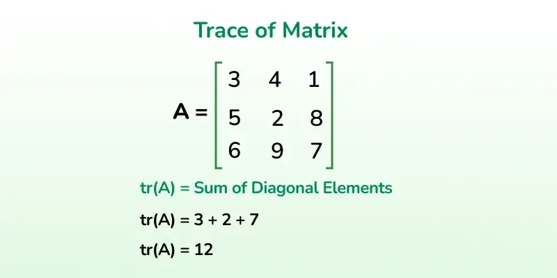
**Trace of a Matrix: Let A = [aij]n × n is a square matrix of order n, then the sum of diagonal elements is called the trace of a matrix which is denoted by tr(A).
**tr(A) = a 11 + a 22 + a 33 + ……….+ a nn
Remember trace of a matrix is also equal to the sum of eigen value of the matrix. For example:
**Properties of Trace of Matrix:
Let A and B be any two square matrices of order n, then
- tr(kA) = k tr(A) where k is a scalar.
- tr(A+B) = tr(A)+tr(B)
- tr(A-B) = tr(A)-tr(B)
- tr(AB) = tr(BA)
**Determinant of Matrices
Determinant represents the scaling factor of the linear transformation associated with the matrix. For example, in a 2 × 2 matrix, the determinant represents the area scaling factor.
**Properties of Determinant
- det(AT) = det(A)
- det(AB) = det(A) × det(B)
- det(kA) = kn × det(A)
- det(A) = 0 implies A is singular.
- |adj(adj(A))| = \mid A \mid^{{(n-1)}^2}
- If we interchange the row or column in determinant its sign changes from positive to negative.
**Rank of a Matrix: Rank of matrix is the number of non-zero rows in the row reduced form or the maximum number of independent rows or the maximum number of independent columns. Rank is denoted as rank(A) or ρ(A). if A is a non-singular matrix of order n, then rank of A = n i.e. ρ(A) = n.
Let A be any m × n matrix and it has square sub-matrices of different orders. A matrix is said to be of rank r, if it satisfies the following properties:
- It has at least one square sub-matrices of order r who has non-zero determinant.
- All the determinants of square sub-matrices of order (r+1) or higher than r are zero.
**Properties of Rank of a Matrix
- If A is a null matrix then ρ(A) = 0 i.e. Rank of null matrix is zero.
- If In is the n × n unit matrix then ρ(A) = n.
- Rank of a matrix A m × n , ρ(A) ≤ min(m,n). Thus ρ(A) ≤m and ρ(A) ≤ n.
- ρ(A n × n ) = n if |A| ≠ 0
- If ρ(A) = m and ρ(B)=n then ρ(AB) ≤ min(m,n).
- If A and B are square matrices of order n then ρ(AB) ≥ ρ(A) + ρ(B) – n.
- If Am×1 is a non zero column matrix and B1×n is a non zero row matrix then ρ(AB) = 1.
- The rank of a skew symmetric matrix cannot be equal to one.
**Solution of a System of Linear Equations
Linear equations can have three kind of possible solutions:
- No Solution
- Unique Solution
- Infinite Solution
**System of homogeneous linear equations AX = 0.
- X = 0. is always a solution; means all the unknowns has same value as zero. (This is also called trivial solution)
- If ρ(A) = number of unknowns, unique solution.
- If ρ(A) < number of unknowns, infinite number of solutions.
**System of non-homogeneous linear equations AX = B.
- If ρ[A:B] ≠ ρ(A), No solution.
- If P[A:B] = ρ(A) = the number of unknown variables, unique solution.
- If ρ[A:B] = ρ(A) ≠ number of unknown, infinite number of solutions.
Here ρ[A:B] is rank of gauss elimination representation of AX = B.
There are two states of the Linear equation system:
- **Consistent State: A System of equations having one or more solutions is called a consistent system of equations.
- **Inconsistent State: A System of equations having no solutions is called inconsistent system of equations.
**Linear dependence and Linear independence of Vector:
- **Linear Dependence: A set of vectors X1, X2, . . ., Xr is said to be linearly dependent if there exist r scalars k1 ,k2, . . ., kr such that: k1 X1 + k2X2 + . . . + kr Xr = 0.
- **Linear Independence: A set of vectors X1 ,X2, . . ., Xr is said to be linearly independent if for all r scalars k1, k2 , . . ., kr such that k1X1 + k2 X2 + . . . + krXr = 0, then k1 = k2 =……. = kr = 0.
**How to Determine Linear Dependency and Independency
Let X1, X2 ….Xr be the given vectors. Construct a matrix with the given vectors as its rows.
- If the rank of the matrix of the given vectors is less than the number of vectors, then the vectors are linearly dependent.
- If the rank of the matrix of the given vectors is equal to the number of vectors, then the vectors are linearly independent.
Eigen Value and Eigen Vector
Eigen vector of a matrix A is a vector represented by a matrix X such that when X is multiplied with matrix A, then the direction of the resultant matrix remains the same as vector X.
Mathematically, above statement can be represented as:
**AX = λX
Where A is any arbitrary matrix, λ are eigen values and X is an eigen vector corresponding to each eigen value.
Here, we can see that AX is parallel to X. So, X is an eigen vector.
**How to Find Eigenvalues and Eigen Vectors of Given Matrices
We know that,
AX = λX
AX – λX = 0
(A – λI) X = 0 . . . (1)
Above condition will be true only if (A – λI) is singular. That means,
|A – λI| = 0 . . . (2)
This is known as characteristic equation of the matrix and the roots of the characteristic equation are the eigen values of the matrix A.
**Properties of Eigen Values
- Eigen values of real symmetric and hermitian matrices are real.
- Eigen values of real skew symmetric and skew hermitian matrices are either pure imaginary or zero.
- Eigen values of unitary and orthogonal matrices are of unit modulus |λ| = 1.
- If λ1 = λ2 = . . . = λn are the eigen values of A, then kλ1, kλ2 . . . kλn are eigen values of kA.
- If λ1, λ2 . . . λn are the eigen values of A, then 1/λ1, 1/λ2 . . . 1/λn are eigen values of A-1.
- If λ1, λ2 . . . λn are the eigen values of A, then λ1k, λ2k . . . λnk are eigen values of Ak.
- Eigen values of A = Eigen Values of AT (Transpose).
- Sum of Eigen Values = Trace of A (Sum of diagonal elements of A).
- Product of Eigen Values = |A|.
- Maximum number of distinct eigen values of A = Size of A.
- If A and B are two matrices of same order then, Eigen values of AB = Eigen values of BA.
LU Decomposition
**LU Decomposition (also known as LU Factorization) is a method used to solve a system of linear equations. It decomposes a given square matrix **A into the product of two matrices **L (Lower Triangular Matrix) and **U (Upper Triangular Matrix), such that:
A = L ⋅ U
Where:
- L is a lower triangular matrix with ones on the diagonal.
- U is an upper triangular matrix.
Probability and Statistics
Probability
Probability refers to the extent of occurrence of events. When an event occurs like throwing a ball, picking a card from deck, etc ., then the must be some probability associated with that event.
**Basic Terminologies:
**Sample Space (S): The set of all possible outcomes of an experiment.
**Event (E): Any subset of the sample space.
**Probability of an Event (P(E)): A measure of the likelihood of an event occurring, where 0≤P(E)≤10 \leq P(E) \leq 10≤P(E)≤1.
- P(S)=1P(S) = 1P(S)=1 (for the sample space).
- P(∅)=0P(\emptyset) = 0P(∅)=0 (for the empty set).
**Important Rules:
**Addition Rule:
- For two mutually exclusive events A and B: P(A∪B) = P(A) + P(B).
- For two non-mutually exclusive events A and B: P(A∪B) = P(A) + P(B) − P(A∩B).
**Multiplication Rule:
- For independent events A and B: P(A∩B) = P(A) ⋅ P(B).
- For conditional probability: P(A∣B) = P(A∩B)/P(B), provided P(B) > 0.
**Events in Probaility
Events are subsets of a sample space and represent the outcomes or collections of outcomes of a random experiment.
**Types of Events
- **Simple Event: Contains a single outcome.
- **Compound Event: Contains multiple outcomes.
- **Sure Event: The entire sample space and it always occurs.
- **Impossible Event: An empty set, ∅ as it never occurs.
- **Mutually Exclusive Events: Events that cannot occur simultaneously.
- **Exhaustive Events: A set of events is exhaustive if their union covers the entire sample space.
- **Independent Events: Two events are independent if the occurrence of one does not affect the probability of the other.
- **Dependent Events: Events where the occurrence of one affects the probability of the other.
**Theorems: General - Let A, B, C are the events associated with a random experiment, then
- P(A∪B) = P(A) + P(B) - P(A∩B)
- P(A∪B) = P(A) + P(B) if A and B are mutually exclusive
- P(A∪B∪C) = P(A) + P(B) + P(C) - P(A∩B) - P(B∩C)- P(C∩A) + P(A∩B∩C)
- P(A∩B') = P(A) - P(A∩B)
- P(A'∩B) = P(B) - P(A∩B)
**Extension of Multiplication Theorem: Let A1, A2, . . . , An are n events associated with a random experiment, then P(A1 ∩ A2 ∩ A3 . . . ∩ An) = P(A1)P(A2/A1)P(A3/A2∩A1) . . . P(An/A1∩A2∩A3∩ . . . ∩An-1)
**Total Law of Probability: Let S be the sample space associated with a random experiment and E1, E2, . . . , En be n mutually exclusive and exhaustive events associated with the random experiment . If A is any event which occurs with E1 or E2 or . . . or En, then
P(A) = P(E1)P(A/E1) + P(E2)P(A/E2) + ... + P(En)P(A/En)
**Conditional Probability: Conditional probability P(A | B) indicates the probability of event 'A' happening given that event B happened.
P(A|B) = \frac{P(A \cap B)}{P(B)}
**Product Rule: Derived from above definition of conditional probability by multiplying both sides with P(B)
P(A ∩ B) = P(B) × P(A|B)
**Bayes's Formula****:** If A1, A2, . . . , An are mutually exclusive and exhaustive events:
P(A_k|B) = \frac{P(B|A_k) P(A_k)}{\sum_{i=1}^n P(B|A_i) P(A_i)}
**Random Variables
A random variable is basically a function which maps from the set of sample space to set of real numbers.
**Discrete Random Variable: Takes finite or countably infinite values.
**Example: Number of heads in n coin tosses.
**Continuous Random Variable: Takes values in an interval.
**Example: Time taken to complete a task.
**Probability Distribution
A Probability Distribution describes how probabilities are assigned to outcomes or ranges of outcomes for a random variable.
**Probability Mass Function (PMF)
Used for discrete random variables.
- P(X = x) = f(x), where f(x) satisfies:
- 0 ≤ f(x) ≤ 1,
- \sum_x f(x) = 1
**Probability Density Function (PDF)
- Used for continuous random variables.
- f(x) \geq 0, \quad \int_{-\infty}^\infty f(x) \, dx = 1
- Probability for a range P(a \leq X \leq b) = \int_a^b f(x) \, dx.
**Cumulative Distribution Function (CDF)
For both discrete and continuous random variables.
F(x) = P(X ≤ x)
- For discrete X: F(x) = \sum_{x_i \leq x} P(X = x_i).
- For continuous X: F(x) = \int_{-\infty}^x f(t) \, dt
**Expected Value (Mean):
- Discrete: E[X] = \sum x_i P(X = x_i).
- Continuous: E[X] = \int_{-\infty}^\infty x f(x) \, dx.
- **Variance: Var(X) = E[X2] - (E[X])2
- **Standard Deviation: \sigma = \sqrt{\text{Var}(X)}.
**Important Distributions
**Binomial Distribution: Binomial Distribution is used to calculate the probability of a specific number of successes in a fixed number of independent trials
- For n independent trials with success probability p:
P(X = k) = \binom{n}{k} p^k (1-p)^{n-k}, \quad k = 0, 1, \dots, n
Mean: E[X] = np, Variance: Var(X) = np(1 − p).
**Poisson Distribution: Poisson Distribution is a discrete probability distribution that models the number of events occurring
- For rare events with rate λ:
P(X = k) = \frac{\lambda^k e^{-\lambda}}{k!}, \quad k = 0, 1, 2, \dots
Mean and Variance: E[X] = Var(X) = λ.
- Continuous distribution over [a, b]:
f(x) = 1/(b−a), a ≤ x ≤ b
Mean: E[X] = (a + b)/2, Variance: Var(X) = (b − a)2/12.
- Bell-shaped curve with parameters μ (mean) and σ2 (Varience):
f(x) = \frac{1}{\sqrt{2\pi \sigma^2}} e^{-\frac{(x-\mu)^2}{2\sigma^2}}
68% of values lie within μ ± σ, 95% within μ ± 2σ.
**Exponential Distribution: For a positive real number \lambda the probability density function of a Exponentially distributed Random variable is given by:
f_X(x) =\begin{cases} \lambda e^{-\lambda x} & if x\in R_X \\ 0 & if x \notin R_X \end{cases}
Where Rx is exponential random variables.
Mean = 1/λ and Variance = 1/λ2
Statistics
Descriptive Statistics: It is a simple tools that help us understand and summarize data.
**Measures of Central Tendency:
- **Mean: Average of the dataset.
- **Median: Middle value when the data is sorted.
- **Mode: Most frequently occurring value in the dataset.
**Measures of Spread:
- **Range: Difference between the maximum and minimum values.
- **Variance and Standard Deviation: Measures of how much the data deviates from the mean.
**Inferential Statistics
- **Sampling Distribution: A probability distribution of a statistic (like the sample mean) obtained through repeated sampling.
- **Central Limit Theorem (CLT): States that the sampling distribution of the sample mean approaches a normal distribution as the sample size increases, regardless of the population's distribution.
Calculus
**Existence of Limit: The **limits of a function f(x) at x = a exists only when its left hand limit and right hand limit exist and are equal i.e. \lim_{x\to a^-}f(x) = \lim_{x\to a^+}f(x)
Also Read **Formal Definition of Limit.
**Some Common Limits:
\bullet\: \lim_{x\to 0} \frac{\sin x}{x} = 1 \hspace{0.5cm} \\\bullet\: \lim_{x\to 0} \cos x = 1 \hspace{0.5cm} \\\bullet\: \lim_{x\to 0} \frac{\tan x}{x} = 1 \\ \bullet\: \lim_{x\to 0} \frac{1-\cos x}{x} = 0 \hspace{0.5cm}\\ \bullet\: \lim_{x\to 0} \frac{\sin x^\circ}{x} = \frac{\pi}{180} \hspace{0.5cm} \\\bullet\: \lim_{x\to a} \frac{x^n - a^n}{x-a} = na^{n-1} \\ \bullet\: \lim_{x\to \infty} \left(1+\frac{k}{x}\right)^{mx} = e^{mk} \hspace{0.5cm}\\ \bullet\: \lim_{x\to 0} (1+x)^{\frac{1}{x}} = e \hspace{0.5cm} \\\bullet\: \lim_{x\to 0} \frac{a^x-1}{x} = \ln a \\ \bullet\: \lim_{x\to 0} \frac{e^x-1}{x} = 1 \hspace{0.5cm} \\\bullet\: \lim_{x\to 0} \frac{\ln (1+x)}{x} = 1 \hspace{0.5cm} \\\bullet\: \lim_{x\to \infty} x^{\frac{1}{x}} = 1\\
Read More about **Properties of Limits.
**L'Hospital Rule:
If the given limit \lim_{x\to a} \frac{f(x)}{g(x)} is of the form \frac{0}{0} or \frac{\infty}{\infty} i.e. both f(x) and g(x) are either 0 or ∞, then the limit can be solved by **L'Hospital Rule.
If the limit is of the form described above, then the L'Hospital Rule says that:
\lim_{x\to a}\frac{f(x)}{g(x)} = \lim_{x\to a}\frac{f^\prime(x)}{g^\prime(x)}
Where f'(x) and g'(x) obtained by differentiating f(x) and g(x). If after differentiating, the form still exists, then the rule can be applied continuously until the form is changed.
A function is said to be continuous over a range if it's graph is a single unbroken curve. Formally, a real valued function f(x) is said to be continuous at a point x = x0 in the domain if: \lim_{x\to x_\circ} f(x) exists and is equal to f(x0).
If a function f(x) is continuous at x = x0 then:
\lim_{x\to x_\circ ^+} f(x) = \lim_{x\to x_\circ ^-} f(x) = \lim_{x\to x_\circ} f(x)
Functions that are not continuous are said to be discontinuous.
Also Read about **Continuity at a Point.
**Differentiability:
The derivative of a real valued function f(x) wrt x is the function f'(x) and is defined as:
\lim_{h\to 0} \frac{f(x+h)-f(x)}{h}
A function is said to be differentiable if the derivative of the function exists at all points of its domain. For checking the differentiability of a function at point x = c, \lim_{h\to 0} \frac{f(c+h)-f(c)}{h}
must exist.
**Note: If a function is differentiable at a point, then it is also continuous at that point, but if a function is continuous at a point does not imply that the function is also differentiable at that point. For example, f(x) = |x| is continuous at x = 0 but it is not differentiable at that point.
**Lagrange’s Mean Value Theorem:
**Suppose f:[a,b]\rightarrow R be a function satisfying three conditions:
- f(x) is continuous in the closed interval a ≤ x ≤ b
- f(x) is differentiable in the open interval a < x < b
Then according to Lagrange's Theorem, there exists at least one point 'c' in the open interval (a, b) such that:
f'(c)=\frac{f(b)-f(a)}{b-a}
**Rolle’s Mean Value Theorem:
Suppose f(x) be a function satisfying three conditions:
- f(x) is continuous in the closed interval a ≤ x ≤ b
- f(x) is differentiable in the open interval a < x < b
- f(a) = f(b)
Then according to Rolle's Theorem, there exists at least one point 'c' in the open interval (a, b) such that:
f '(c) = 0
**Differentiation Formulas
Some of the most common formula used to find derivative are tabulated below:
| d/dx(c) | 0 |
|---|---|
| d/dx{c.f(x)} | c.f'(x) |
| d/dx(x) | 1 |
| d/dx(xn) | nxn-1 |
| d/dx{f(g(x))} | f'(g(x)).g'(x) |
| d/dx(ax) | ax.ln(a) |
| d/dx{ln(x)} {Note: ln(x) = loge(x)} | 1/x, x>0 |
| d/dx(logax) | 1/xln(a) |
| d/dx(ex) | ex |
| d/dx{sin(x)} | cos(x) |
| d/dx{cos(x)} | -sin(x) |
| d/dx{tan(x)} | sec2x |
| d/dx{sec(x)} | sec(x).tan(x) |
| d/dx{cosec(x)} | -cosec(x).cot(x) |
| d/dx{cot(x)} | -cosec2(x) |
| d/dx{sin-1(x)} | 1/√(1 - x2) |
| d/dx{cos-1(x)} | -1/√(1 - x2) |
| d/dx{tan-1(x)} | 1/(1+x2) |
Maxima and Minima
- **Critical Points: Points where the derivative f′(x) = 0 or f′(x) is undefined.
- **Local Maximum: f(x) has a local maximum at x = c if f(c) ≥ f(x) for all x in a small neighborhood around c.
- **Local Minimum: f(x) has a local minimum at x = c if f(c) ≤ f(x) for all x in a small neighborhood around c.
- **Global Maximum/Minimum: The highest/lowest value of f(x) over its entire domain.
Read More about **Maxima and Minima.
**First Derivative Test****:**
If f′(x) changes:
- From positive to negative at x = c: Local Maximum at c.
- From negative to positive at x = c: Local Minimum at c.
- If no change: x = c is a point of inflection.
**Second Derivative Test:
Compute the second derivative f′′(x):
- If f′′(c) > 0: Local Minimum at c.
- If f′′(c) < 0: Local Maximum at c.
- If f′′(c) = 0: Test is inconclusive (use the first derivative test or higher-order derivatives).
**Concavity:
f(x) is:
- Concave Up if f′′(x) > 0.
- Concave Down if f′′(x) < 0.
Point of inflection: f(x) changes concavity (where f′′(x) = 0.
**Maxima and Minima in Multivariable Functions****:**
For f(x, y):
**Critical Points: Solve ∂f/∂x = 0 and ∂f/∂y = 0.
**Second **Partial Derivatives: Compute:
- fxx = ∂2f/∂x2,
- fyy = ∂2f/∂y2,
- fxy = ∂2f/∂x∂y.
**Hessian Determinant: H = fxxfyy − (fxy)2.
- If H > 0 and fxx > 0: Local Minimum.
- If H > 0 and fxx < 0: Local Maximum.
- If H < 0: Saddle Point.
- If H = 0: Test is inconclusive.
**Integrals
Integrals can be classified as:
- **Definite Integral
- **Indefinite Integral
- **Improper Integrals
**Indefinite Integrals:
Let f(x) be a function. Then the family of all its antiderivatives is called the indefinite integral of a function f(x) and it is denoted by ∫f(x)dx.
- The symbol ∫f(x)dx is read as the indefinite integral of f(x) with respect to x. Thus ∫f(x)dx= ∅(x) + C. Thus, the process of finding the indefinite integral of a function is called integration of the function.
**Fundamental Integration Formulas:
Some common integration formulas include:
- ∫xndx = (xn+1/(n+1))+C
- ∫(1/x)dx = (loge|x|)+C
- ∫exdx = (ex)+C
- ∫axdx = ((ax)/(logea))+C
- ∫sin(x)dx = -cos(x)+C
- ∫cos(x)dx = sin(x)+C
- ∫sec2(x)dx = tan(x)+C
- ∫cosec2(x)dx = -cot(x)+C
- ∫sec(x)tan(x)dx = sec(x)+C
- ∫cosec(x)cot(x)dx = -cosec(x)+C
- ∫cot(x)dx = log|sin(x)|+C
- ∫tan(x)dx = log|sec(x)|+C
- ∫sec(x)dx = log|sec(x)+tan(x)|+C
- ∫cosec(x)dx = log|cosec(x)-cot(x)|+C
**Definite Integrals:
Definite integrals are the extension after indefinite integrals, definite integrals have limits [a, b]. It gives the area of a curve bounded between given limits.
\int_{a}^{b}F(x)dx, it denotes the area of curve F(x) bounded between a and b, where a is the lower limit and b is the upper limit.
**Note: If f is a continuous function defined on the closed interval [a, b] and F be an anti derivative of f. Then \int_{a}^{b}f(x)dx= \left [ F(x) \right ]_{a}^{b} = F(a) - F(b).
Here, the function f needs to be well defined and continuous in [a, b].
- \int_{a}^{b}f(x)dx=\int_{a}^{b}f(t)dt
- \int_{a}^{b}f(x)dx=-\int_{b}^{a}f(x)dx
- \int_{a}^{b}f(x)dx=\int_{a}^{c}f(x)dx+\int_{c}^{b}f(x)dx
- \int_{a}^{b}f(x)=\int_{a}^{b}f(a+b-x)dx
- \int_{0}^{b}f(x)=\int_{0}^{b}f(b-x)dx
- \int_{0}^{2a}f(x)dx=\int_{0}^{a}f(x)dx+\int_{0}^{a}f(2a-x)dx
- \int_{-a}^{a}f(x)dx=2\int_{0}^{a}f(x)dx, if f(x) is even function i.e f(x) = f(-x)
- \int_{-a}^{a}f(x)dx=0, if f(x) is odd function
**Newton-Leibnitz Rule
For a definite integral F(x) = \int_{a(x)}^{b(x)} f(t) \, dt:
\frac{d}{dx} \left[ \int_{a(x)}^{b(x)} f(t) \, dt \right] = f(b(x)) \cdot b'(x) - f(a(x)) \cdot a'(x)
Application of Integrals
- Area Under a Curve
- Area Between Curves
- Area Between Polar Curves
- Arc Length of Curves
- Volume of Solids of Revolution
- Surface Area of Revolution
**Area Under a Curve
The area enclosed between a curve y = f(x), the x-axis, and the limits x = a and x = b is:
\text{Area} = \int_a^b f(x) \, dx
- If f(x) < 0, take the absolute value of the integral.
**Between Two Curves
The area between two curves y = f(x) and y = g(x) from x = a to x = b is:
Area = \int_a^b \big| f(x) - g(x) \big| \, dx.
**Length of a Curve
The length of a curve y = f(x) from x = a to x = b is:
Length = \int_a^b \sqrt{1 + \left( \frac{dy}{dx} \right)^2} \, dx
For parametric equations x = x(t), y = y(t), the arc length is:
Length = \int_{t_1}^{t_2} \sqrt{\left( \frac{dx}{dt} \right)^2 + \left( \frac{dy}{dt} \right)^2} \, dt
**Volume of Solids of Revolution
**Disk Method: When a curve y = f(x) is revolved about the x-axis: Volume = \pi \int_a^b \left[ f(x) \right]^2 \, dx
**Shell Method: When a curve y = f(x) is revolved about the y-axis: Volume = 2\pi \int_a^b x \cdot f(x) \, dx.
For parametric equations x = x(t), y = y(t):
- Revolved about x-axis: Volume = \pi \int_{t_1}^{t_2} \left[ y(t) \right]^2 \frac{dx}{dt} \, dt
**Surface Area of Solids of Revolution
- **Revolution about the x-axis:Surface Area = 2\pi \int_a^b f(x) \sqrt{1 + \left( \frac{dy}{dx} \right)^2} \, dx
- **Revolution about the y-axis: Surface Area = 2\pi \int_a^b x \sqrt{1 + \left( \frac{dy}{dx} \right)^2} \, dx