Last Minute Notes DBMS (original) (raw)

Last Updated : 10 Jan, 2026

A Database Management System is an organized collection of interrelated data that helps in accessing data quickly, along with efficient insertion and deletion of data into the DBMS. DBMS organizes data in the form of tables, schemas, records, etc.

**DBMS over File System

The file system has numerous issues, which were resolved with the help of DBMS. The issues with the file system are:

**Physical Access Management: Users are responsible for managing the physical details required to access the database.
**File System Suitability: File systems are effective for handling small databases but lack efficiency for larger ones.
**Concurrency Issues: For large databases, the operating system struggles to manage concurrency effectively, leading to potential conflicts.
**Single-User Access: In a file system, only one user can access the entire dataset at a time, limiting scalability and multi-user functionality.
**Data access: In a file system, accessing data was difficult and insecure as well. Accessing data concurrently was not possible.
**No Backup and Recovery: There is no backup and recovery in the file system, which can lead to data loss.

ER-Model

**ER Diagram

An ER diagram is a model of a logical view of the database which is represented using the following components:

components_of_er_diagram

**Entity: The entity is a real-world object, represented using a rectangular box.

**Strong Entity: A strong entity set has a primary key and all the tuples of the set can be identified using that primary key
**Weak entity: When an entity does not have sufficient attributes to form a primary key. Weak entities are associated with another strong entity set also known as identifying an entity. A weak entity's existence depends upon the existence of its identifying entity. The weak entity is represented using a double-lined or bold-lined rectangle.

**Attribute: Attribute is the properties or characteristics of the real-world object. It is represented using an oval.

**Key attribute: The attribute which determines each entity uniquely is known as the Key attribute. It is represented by an oval with an underlying line.
**Composite Attribute: An attribute that is composed of many other attributes. E.g. address is an attribute it is formed of other attributes like state, district, city, street, etc. It is represented using an oval comprises of many other ovals.
**Multivalued Attribute: An attribute that can have multiple values, like a mobile number. It is represented using a double-lined oval.
**Derived attribute: An attribute that can be derived from other attributes. E.g. Age is an attribute that can be derived from another attribute Data of Birth. It is represented using a dashed oval.

**Relationship: A relationship is an association between two or more entities. Entities are connected or related to each other and this relationship is represented using a diamond.

**Participation Constraint: It specifies the maximum or a minimum number of relationship instances in which any entity can participate. In simple words, participation means how an entity is linked to a relationship.

**Total Participation: Every entity in the entity set participates in at least one relationship in the relationship set.
**Example:
In the "Manages" relationship between Emp (Employee) and Dept (Department):
If every department must have a manager, then Dept has total participation in the "Manages" relationship.
**Partial Participation: Some entities in the entity set participate in the relationship, but not all.
**Example:
In the same "Manages" relationship:
If not all employees are managers, then Emp has partial participation in the "Manages" relationship.

**Cardinality in DBMS

Cardinality of relation expresses the maximum number of possible relationship occurrences for an entity participating in a relationship. Cardinality of a relationship can be defined as the number of times an entity of an entity set participates in a relationship set. Let's suppose a binary relationship R between two entity sets A and B. The relationship must have one of the following mapping cardinalities:

**One-to-One: When one entity of A is related to at most one entity of B, and vice-versa.
**One-to-Many: When one entity of A is related to one or more than one entity of B. Whereas B is associated with at most one entity in A.
**Many-to-One: When one entity of B is related to one or more than one entity of A. Whereas A is associated with at most one entity in B.
**Many-to-Many: Any number of entities of A is related to any number of entities of B, and vice-versa.

The most commonly asked question in ER diagram is the minimum number of tables required for a given ER diagram. Generally, the following criteria are used:

**Cardinality	**Minimum No. of tables
1:1 cardinality with partial participation of both entities	2
1:1 cardinality with a total participation of at least 1 entity	1
1:n cardinality	2
m:n cardinality	3

If the relation is one-to-many or many-to-one then two or more relational tables can be combined.
If the relation is many-to-many two tables cannot be combined.
If the relation is one-to-one and there is total participation of one entity then that entity can be combined with a relational table.
If there is total participation of both entities then one table can be obtained by combining one table and both entities of the relation.

**Note: This is a general observation. Special cases need to be taken care of. We may need an extra table if the attribute of a relationship can't be moved to any entity side.

**Specialization: It is a top-down approach in which one entity is divided/specialized into two or more sub-entities based on its characteristics.

**Generalization: It is a bottom-up approach in which common properties of two or more sub-entities are combined/generalized to form one entity. It is exactly the reverse of Specialization. In this, two or lower level entities are generalized to one higher level entity.

**Aggregation: Aggregation is an abstraction process through which relationships are represented as higher-level entity sets.

mapping_cardinalities_3

Read more about Introduction to ER Model.

Database Design

Database design goals are:

To have zero redundancy in the system
Loss-less join
Dependency preservation
Overcome all the shortcomings of conventional file system

According to E.F. Codd (Codd's Rule in DBMS), "All the records of the table must be unique".

Integrity Constraints Of RDBMS

**Integrity constraints are rules that ensure data in a database is accurate and consistent. The main types are:

**Entity Integrity: Each record must have a unique identifier (primary key).
**Referential Integrity: Relationships between tables must be consistent (using foreign keys).
**Domain Integrity: Data in each field must meet certain rules (e.g., correct type or range).
**User-Defined Integrity: Custom rules set by users for specific needs.

Key Terms in Relational Databases

**Table: A collection of rows (records) in a database.
**Record: A single row in a table, containing data fields.
**Field: A column in a table, also called an attribute.
**Domain: The set of possible values a field can have.
**Key: A method for identifying specific records in a table.
**Index: A tool that speeds up database queries and searches.
**View: A virtual table created from data in actual tables.
**Tuple: Another word for a record or row in a table.
**Relation: Another term for a table.
**Cardinality: The total number of rows in a table.
**Degree: The number of columns in a table.
**Schema: The structure of a table, including its name, fields, and allowed values.
**Prime Attributes: Unique attributes used to identify rows, part of the primary or candidate key (e.g., student ID).
**Non-Prime Attributes: Attributes not part of any key, may have duplicates, and provide additional information (e.g., student's first name, date of birth).

Keys in database

**Keys of a relation: There are various types of keys in a relation which are: **primary key, **candidate key, **super key, and **alternate key. Let's take a table called STUDENT

**student_id	**name	**email	**phone
1	Alice	alice@xyz.com	1234567890
2	Bob	bob@xyz.com	9876543210
3	Charlie	charlie@xyz.com	5555555555

**1. Primary Key

The **primary key is the unique identifier for each record. In this case, student_id is the primary key because each student has a unique ID. **Primary Key:student_id

**2. Candidate Key

The minimal set of attributes that can determine a tuple uniquely. There can be more than 1 candidate key of a relation and its proper subset can't determine tuple uniquely and it can't be NULL. In this case, both student_id and email can uniquely identify a student. **Candidate Keys: student_id, email, phone.

**3. Super Key

A **super key is any combination of columns that uniquely identifies a record. It can include extra attributes beyond what is necessary for uniqueness. A candidate key is always a super key but vice versa is not true. For example, student_id combined with phone or email would still uniquely identify a student. **Super Keys: student_id, student_id + phone, email + phone etc.

**4. Alternate Key

An **alternate key is any candidate key that is not chosen as the primary key. In this case, since student_id is the primary key, email becomes the alternate key.**Alternate Key: email, phone.

**5. Foreign Key

Foreign Key is a set of attributes in a table that is used to refer to the primary key or alternative key of the same or another table.

foreign_key

Functional Dependency

It is a constraint that specifies the association/ relationship between a set of attributes. It is represented as A->B, where set A can determine the values of set B correctly. The A is known as the **Determinant, and B is known as the **Dependent.

**Types of Functional Dependencies in DBMS:

Functional Dependencies in DBMS define the relationship between attributes in a database, where one set of attributes uniquely determines another set.

**Trivial Functional Dependency: A functional dependency where the right-hand side is a subset of the left-hand side.
**Example:A → A (any attribute depends on itself).
**Non-Trivial Functional Dependency: A functional dependency where the right-hand side is not a subset of the left-hand side.
**Example:Student_ID → Student_Name (Student_ID determines Student_Name).
**Multivalued Functional Dependency: When one attribute determines a set of values for another attribute, but not directly.
**Example:Student_ID →→ Student_Courses (A student may have multiple courses).
**Transitive Functional Dependency:
When one attribute depends on another through a third attribute.
**Example:Student_ID → Student_Name and Student_Name → Department, so Student_ID → Department.

All dependencies can relate to a Student table where Student_ID is the key.

**Armstrong's Axioms: It is a statement that is always considered true and used as a starting point for further arguments. Armstrong axiom is used to generate a closure set in a relational database.

Armstrong Axiom

**Attribute Closure(X + ):All attributes of the set are functionally determined by X.

**Prime Attribute: An attribute that is part of one candidate key.
**Non-prime Attribute: An attribute that is not a part of any candidate key.

**Example: If the relation R(ABCD) {A->B, B->C, C->D}, then the attribute closure of

A will be (A+)={ABCD} [A can determine B, B can determine C, C can determine D]
B will be (B+)={BCD} [B can determine C, C can determine D]
C will be (C+)={CD} [C can determine D]
D will be (D+)={D} [D can determine itself]

Note: With the help of Attribute closure, we can easily determine the Superkey [__The set of attributes whose closure contains all attributes of a relation_] of a relation, So in the above example A is the superkey of the given relation. There can be more than one superkey in a relationship.

**Example: If the relation R(ABCDE) {A->BC, CD->E, B->D, E->A}, then the attribute closure will be

A+= {ABCDE}
B+= {BD}
C+= {C}
D+= {D}
E+= {ABCDE}

Steps to Find a Candidate Key (Minimal Super Key)

**Identify all Super Keys:
A super key is any set of attributes that can uniquely identify a record. Start by considering combinations of attributes that can act as super keys.
**Remove Redundant Attributes:
Check if any attribute in the super key is unnecessary. If removing an attribute still allows the set to uniquely identify records, it is redundant. Continue removing until no more attributes can be removed without losing uniqueness.
**Minimal Super Key = Candidate Key:
After eliminating unnecessary attributes, the resulting set is a **Candidate Key.

**Equivalence sets of Functional Dependency

If two sets of a functional dependency are equivalent, i.e. if A+= B+. Every FD in A can be inferred from B, and every FD in B can be inferred from A, then A and B are functionally equivalent.

**Minimal Cover or Canonical Cover

A **minimal cover is the smallest set of functional dependencies that preserves the same information.
Steps:

**Single attribute on the right-hand side: Break dependencies like AB → C into AB → B and AB → C.
**Remove unnecessary attributes: Eliminate attributes on the left-hand side if not needed.
**Remove redundant dependencies: If a dependency is implied by others, remove it.

**Example: Given: AB → C, A → B, BC → A, Minimal cover could be: A → B, B → C, BC → A.

**Normalization: Normalization is used to eliminate the following anomalies:

**Insertion Anomaly
**Deletion Anomaly
**Updation Anomaly

Normalization was introduced to achieve integrity in the database and make the database more maintainable.

Normal Forms

**1. First Normal Form: A relation is in first normal form if it does not contain any multi-valued or composite attribute. If the data is in 1NF then it will have high redundancy. First Normal Form (1NF) is considered the default state for any relational table.

**2. Second Normal Form: A relation is in the second normal form if it is in the first normal form and if it does not contain any partial dependency.

**Partial Dependency: A dependency is called partial dependency if any proper subset of candidate key determines non-prime (which are not part of candidate key) attribute.
Let R be the relational schema and X, Y, A is the set of attributes. Suppose X is any candidate key, Y is a proper subset of candidate key, and A is a Non-prime attribute.

Partial Dependency

Y->A will be partial dependency iff, Y is a proper subset of candidate key, and A is a non-prime attribute.

**Full Functional Dependency: If A and B are an attribute set of a relation, B is fully functional dependent on A, if B is functionally dependent on A but not on any proper subset of A.

**3. Third Normal Form: A relation is in the third normal form if it is in the second normal form and it does not contain any transitive dependency. For a relation to be in Third Normal Form, either LHS of FD should be super key or RHS should be the prime attribute.

**4. Boyce-Codd Normal Form: A relation is inBoyce-CoddNormal Form if the LHS of every FD is super key. The relationship between Normal Forms can be represented as **1NF, 2NF, 3NF or BCNF.

Design Goal	1NF	2NF	3NF	BCNF
Zero Redundancy	High redundancy	Less than 1NF	Less than 2NF	No redundancy
Loss-less decomposition	Always	Always	Always	Always
Dependency preservation	Always	Always	Always	Sometimes Not possible

**Properties of Decomposition:

**Loss-less Join Decomposition: There should not be the generation of any new tuple because of the decomposition.
If [R1 ⋈ R2 ⋈ R3.......⋈ Rn] = R then loss-less join decomposition , If [R1 ⋈ R2 ⋈ R3 ........ ⋈ Rn] ⊃ R then lossy join decomposition.

Consider the relation R(A,B,C) with the functional dependencies: A→B , B→C . Decompose R into R1(A,B) and R2(B,C) :

To check for a lossless join, ensure the common attribute B is a candidate key in at least one of the decomposed relations:

In R1(A,B), A→B, so A is a key.
In R2(B,C), B→C, so B is a key.

When R1 and R2 are joined on B, no information is lost. Therefore, the decomposition is lossless.

**Dependency Preserving Decomposition: There should not be the loss of any tuple because of the decomposition. Let R be a relation with Functional dependency F. After decomposition R is decomposed into R1, R2, R3......Rn with FD set F1, F2, F3......Fn respectively. If F1, F2, F3.....Fn ≣ F, then the decomposition is dependency preserving otherwise not.

Suppose we have a relation R(A,B,C) with the functional dependencies: A→B , B→C. If we decompose R into R1(A,B) and R2(B,C) :

R1 preserves the dependency A→B.
R2 preserves the dependency B→C.

Since all original functional dependencies are preserved in at least one of the decomposed relations, dependency preservation is achieved.

Data Retrieval (SQL, RA)

**Commands to Access Database: For efficient data retrieval, insertion, deletion, updation, etc. The commands in the Database are categorized into three categories, which are as follows:

**DDL [Data Definition language]: It deals with how data should store in the database. DDL commands include CREATE, ALTER, DROP, COMMENT, and TRUNCATE
**DML [Data Manipulation language]: It deals with data manipulation like modifying, updating, deleting, etc. DML commands include SELECT, INSERT, DELETE, UPDATE, MERGE AND CALL.
**DCL [Data Control Language]: It acts as an access specifier, and includes GRANT, AND REVOKE.

**Query Language: Language using which any user can retrieve some data from the database.

**Note: Relational model is a theoretical framework RDBMS is its implementation.

**Relational Algebra: Procedural language with basic and extended operators.

Return those tuples which are either in R1 or R2.

Maximum number of rows returned **= m+n
Minimum number of rows returned = **max(m,n)

**Basic Operator	**Semantic
σ(Selection)	Select rows based on a given condition
π (Projection)	Project some columns
X (Cross Product/ Cartesian Product)	Cross product of relations, returns ***mn** rows where m and n are numbers of rows in R1 and R2 respectively.
U (Union)
- (Minus)	R1-R2 returns those tuples which are in R1 but not in R2. Maximum number of rows returned = m Minimum number of rows returned = m-n
ρ(Rename)	Renaming a relation to another relation.

**Extended Operator	**Semantic
(Intersection)	Returns those tuples which are in both relation R1 and R2. Maximum number of rows returned = min(m,n) Minimum number of rows returned = 0
⋈(Conditional Join)	Selection from two or more tables based on some condition (Cross product followed by selection)
⋈(Equi Join)	It is a special case of conditional join when only an equality condition is applied between attributes.
⋈(Natural Join)	In natural join, equality condition on common attributes holds, and duplicate attributes are removed by default. **Note: Natural Join is equivalent to the cross product of two relations have no attribute in common and the natural join of a relation R with itself will return R only.
⟕(Left Outer Join)	When applying join on two relations R and S, Left Outer Joins gives all tuples of R in the result set. The tuples of R which do not satisfy the join condition will have values as NULL for attributes of S.
⟖(Right Outer Join)	In a join operation between R and S, Right Outer Joins gives all tuples of S in the result set. The tuples of S which do not satisfy the join condition will have values as NULL for attributes of R
⟗(Full Outer Join)	While Performing a join on relations R and S, Full Outer Joins gives all tuples of S and all tuples of R in the result set. The tuples of S which do not satisfy the join condition will have values as NULL for attributes of R and vice versa.
/ (Division Operator)	Division operator A/B will return those tuples in A which is associated with every tuple of B.**Note: Attributes of B should be a proper subset of attributes of A. The attributes in A/B will be Attributes of A- Attribute of B.

**Operator	**Meaning
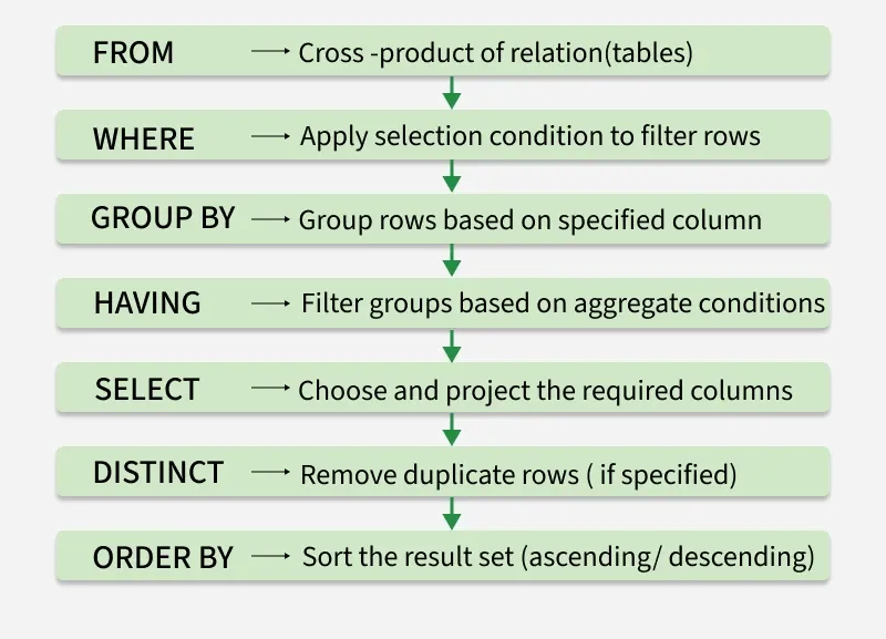
**SELECT	Selects columns from a relation or set of relations. It defines WHAT is to be returned. **Note: As opposed to Relational Algebra, it may give duplicate tuples for the repeated values of an attribute.
**FROM	**FROM is used to define the Table(s) or View(s) used by the SELECT or WHERE statements
**WHERE	**WHERE is used to define what records are to be included in the query. It uses conditional operators.
**EXISTS	**EXISTS is used to check whether the result of a correlated nested query is empty (contains no tuples) or not.
**GROUP BY	**GROUP BY is used to group the tuples based on some attribute or set of attributes like counting the number of students GROUP BY the department.
**ORDER BY	**ORDER BY is used to sort the fetched data in either ascending or descending according to one or more columns.
**Aggregate functions	Find the aggregated value of an attribute. Used mostly with GROUP BY. e.g.; count, sum, min max. ***select count() from the student group by dept_id Note:** we can select only those columns which are part of GROUP BY.
**Nested Queries	When one query is a part of another query.
**UPDATE	It is used to update records in a table.
**DELETE	It is used to delete rows in a table.
**LIKE	LIKE operator is used with the WHERE clause to search a specified pattern in a column.
**IN	IN operator is used to specify multiple values in the WHERE clause.
**BETWEEN	It selects values within a range.
**Aliases	It is used to temporarily rename a table or a column heading.
**HAVING	The HAVING clause was added because the WHERE keyword could be used with aggregate functions.

Execution Flow

dbms

Execution Flow

File Structure

**File organization: It isthe logical relation between records and it defines how file records are mapped into disk blocks(memory). A database is a collection of files, each file is a collection of records, and each record contains a sequence of fields. **The blocking Factor is the average number of records per block.

Strategies for storing files of records in block:

**Spanned Strategy: It allows a partial part of the record to be stored in the block. It is suitable for variable-length records. No wastage of memory in spanned strategy but block access time gets increases.
**Unspanned Strategy: Data cannot be stored partially, the whole block will be occupied, this can lead to internal fragmentation and wastage of memory but block access time is reduced. This is suitable for fixed-length records.

File organizations is of following types:

**Sequential File: In this method, files are stored in sequential order one after another.

**Blocking factor: \left \lfloor \frac{Block\ Size}{Record\ Size} \right \rfloor
**Number of record blocks: \left \lceil \frac{Total\ number\ of\ records}{Blocking\ factor} \right \rceil
**Average number of blocks accessed by linear search: \left \lfloor \frac{number\ of\ record\ blocks}{2} \right \rfloor
**Average number of blocks accessed by binary search: \left \lfloor { log_2 \ number\ of\ record\ blocks} \right \rfloor

**Index File:

**Index blocking factor: \left \lfloor \frac{number\ of\ record\ blocks \ +\ 1}{2} \right \rfloor
**First level index block: \left \lfloor \frac{number\ of\ record\ blocks}{index\ blocking\ factor} \right \rfloor
**Number of block accesses: \left \lfloor { log_2 \ (first\ level\ index\ blocks)} \right \rfloor + 1

**Indexing Type:

**1. Single level Index

**Primary Index(Sparse): A primary index is an ordered file(ordered with key field), records of fixed length with two fields. The first field is the same as the primary key of the data file and the second field is a pointer to a data block, where the key is available. In Sparse indexing, for a set of database records there exists a single entry in the index file.

**Number of index file entries ≤ Number of database records.

**Secondary Index (Dense): Secondary index provides secondary means of accessing a file for which primary access already exists. In Dense indexing, for every database record, there exists an entry in the index file. The index blocking factor is the same for all indexes.

**Number of database records = Number of entries in the index file
**Number of block accesses= \left \lceil{log_2\ ( single\ level\ index\ block)} \right \rceil + 1

**Clustered Index(Sparse): A clustering index is created on a data file whose records are physically ordered on a non-key field (called a Clustering field).Almost one clustering index is possible.

**Single-level index blocks= \left \lceil \frac{Number\ of\ distinct\ values\ over\ non\ key\ field}{Index\ blocking\ factor} \right \rceil + 1
**Number of block accesses= \left \lceil{log_2\ ( single\ level\ index\ block)} \right \rceil + 1

**2. Multilevel Index

**Indexed sequential access method: Second level index is always sparse.

**Level 1 = "first-level index blocks" computed by index
**Level 2 = \left \lceil \frac{Number\ of\ blocks\ in\ level\ (1)}{index\ blocking\ factor} \right \rceil
**Level n = \left \lceil \frac{Number\ of\ blocks\ in\ level\ (n-1)}{index\ blocking\ factor} \right \rceil =1
**Number of blocks = \sum_{i=1}^{n} (Number\ of\ blocks\ in\ level\ i)
**Number of block access = n+1

**B-Tree****:** Also known as Baye's or balanced Search Tree. At every level, we have Key and Data pointers, and data pointer points either block or record.

**Root node: B-tree can have children between **2 and **p, where p is the Order of the tree.
**Internal Node: \left \lceil \frac {n}{2} \right \rceil to n children.
**Leaf nodes all are at the same level.
**Block size = p × (size of block pointer) + (p-1)× (Size of key field + size of record pointer)
**Minimum number of nodes = 1 + (\frac{2[(\frac{p}{2})^h -1]}{(\frac{p}{2}) -2})
**Maximum number of nodes = \frac{p^{h+1}-1}{p-1}
**Minimum height = \left ( \left \lceil log_p \ l \right \rceil \right ) l is the number of leaves
**Maximum height = \left \lfloor 1 +log_{\frac {p}{2}} \frac{l}{2} \right \rfloor

**B + Tree****:** It is the same as B-tree. All the records are available at the leaf (last) level. B+ tree allows both sequential and random access whereas in B-tree only random access was allowed. Each leaf node has one block pointer and all the leaf nodes are connected to the next leaf node using a block pointer.

**Order of non-leaf node= [p × size of block pointer] + [(p-1) × size of key field] <= Block size.
**Order of Leaf node= [(pleaf -1) × (size of key field + size of record pointer) + p × (size of block pointer) <= Block size]

Transaction and Concurrency Control

A transaction is a unit of instruction or set of instructions that performs a logical unit of work. Transaction processes are always atomic in nature either they will execute completely or do not execute.

**Transaction Properties:

**Atomicity: Either execute all operations or none of them. It is managed by the transaction Management Component.
**Consistency: Database must be consistent before and after the execution of the transaction. If atomicity, isolation, and durability are implemented accurately, consistency will be achieved automatically.
**Isolation: In concurrent transactions, the execution of one transaction must not affect the execution of another transaction. It is managed by the Concurrency Control component.
**Durability: After the commit operation, the changes should be durable and persist always in the database. It is managed by the Recovery Management component.

**Transaction States:

A transaction in DBMS goes through various states during its execution to ensure consistency and reliability in the database.

**States of Transactions:

**Active: Transaction is executing its operations.

**Partially Committed: Transaction has completed its final step but is yet to be made permanent.

**Committed: All changes are successfully saved in the database.

**Failed: An error or issue prevents the transaction from completing.

**Aborted: Changes are rolled back, and the transaction is terminated.

**Flow:

dbms_2-22

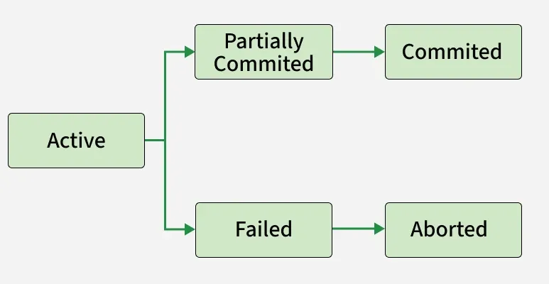
Flow