What’s new in 0.23.0 (May 15, 2018) — pandas 2.2.3 documentation (original) (raw)
This is a major release from 0.22.0 and includes a number of API changes, deprecations, new features, enhancements, and performance improvements along with a large number of bug fixes. We recommend that all users upgrade to this version.
Highlights include:
- Round-trippable JSON format with ‘table’ orient.
- Instantiation from dicts respects order for Python 3.6+.
- Dependent column arguments for assign.
- Merging / sorting on a combination of columns and index levels.
- Extending pandas with custom types.
- Excluding unobserved categories from groupby.
- Changes to make output shape of DataFrame.apply consistent.
Check the API Changes and deprecations before updating.
Warning
Starting January 1, 2019, pandas feature releases will support Python 3 only. See Dropping Python 2.7 for more.
What’s new in v0.23.0
- New features
- JSON read/write round-trippable with orient='table'
- Method .assign() accepts dependent arguments
- Merging on a combination of columns and index levels
- Sorting by a combination of columns and index levels
- Extending pandas with custom types (experimental)
- New observed keyword for excluding unobserved categories in GroupBy
- Rolling/Expanding.apply() accepts raw=False to pass a Series to the function
- DataFrame.interpolate has gained the limit_area kwarg
- Function get_dummies now supports dtype argument
- Timedelta mod method
- Method .rank() handles inf values when NaN are present
- Series.str.cat has gained the join kwarg
- DataFrame.astype performs column-wise conversion to Categorical
- Other enhancements
- Backwards incompatible API changes
- Dependencies have increased minimum versions
- Instantiation from dicts preserves dict insertion order for Python 3.6+
- Deprecate Panel
- pandas.core.common removals
- Changes to make output of DataFrame.apply consistent
- Concatenation will no longer sort
- Build changes
- Index division by zero fills correctly
- Extraction of matching patterns from strings
- Default value for the ordered parameter of CategoricalDtype
- Better pretty-printing of DataFrames in a terminal
- Datetimelike API changes
- Other API changes
- Deprecations
- Removal of prior version deprecations/changes
- Performance improvements
- Documentation changes
- Bug fixes
- Contributors
New features#
JSON read/write round-trippable with orient='table'#
A DataFrame can now be written to and subsequently read back via JSON while preserving metadata through usage of the orient='table' argument (see GH 18912 and GH 9146). Previously, none of the available orient values guaranteed the preservation of dtypes and index names, amongst other metadata.
In [1]: df = pd.DataFrame({'foo': [1, 2, 3, 4], ...: 'bar': ['a', 'b', 'c', 'd'], ...: 'baz': pd.date_range('2018-01-01', freq='d', periods=4), ...: 'qux': pd.Categorical(['a', 'b', 'c', 'c'])}, ...: index=pd.Index(range(4), name='idx')) ...:
In [2]: df
Out[2]:
foo bar baz qux
idx
0 1 a 2018-01-01 a
1 2 b 2018-01-02 b
2 3 c 2018-01-03 c
3 4 d 2018-01-04 c
[4 rows x 4 columns]
In [3]: df.dtypes Out[3]: foo int64 bar object baz datetime64[ns] qux category Length: 4, dtype: object
In [4]: df.to_json('test.json', orient='table')
In [5]: new_df = pd.read_json('test.json', orient='table')
In [6]: new_df
Out[6]:
foo bar baz qux
idx
0 1 a 2018-01-01 a
1 2 b 2018-01-02 b
2 3 c 2018-01-03 c
3 4 d 2018-01-04 c
[4 rows x 4 columns]
In [7]: new_df.dtypes Out[7]: foo int64 bar object baz datetime64[ns] qux category Length: 4, dtype: object
Please note that the string index is not supported with the round trip format, as it is used by default in write_json to indicate a missing index name.
In [8]: df.index.name = 'index'
In [9]: df.to_json('test.json', orient='table')
In [10]: new_df = pd.read_json('test.json', orient='table')
In [11]: new_df Out[11]: foo bar baz qux 0 1 a 2018-01-01 a 1 2 b 2018-01-02 b 2 3 c 2018-01-03 c 3 4 d 2018-01-04 c
[4 rows x 4 columns]
In [12]: new_df.dtypes Out[12]: foo int64 bar object baz datetime64[ns] qux category Length: 4, dtype: object
Method .assign() accepts dependent arguments#
The DataFrame.assign() now accepts dependent keyword arguments for python version later than 3.6 (see also PEP 468). Later keyword arguments may now refer to earlier ones if the argument is a callable. See thedocumentation here (GH 14207)
In [13]: df = pd.DataFrame({'A': [1, 2, 3]})
In [14]: df Out[14]: A 0 1 1 2 2 3
[3 rows x 1 columns]
In [15]: df.assign(B=df.A, C=lambda x: x['A'] + x['B']) Out[15]: A B C 0 1 1 2 1 2 2 4 2 3 3 6
[3 rows x 3 columns]
Warning
This may subtly change the behavior of your code when you’re using .assign() to update an existing column. Previously, callables referring to other variables being updated would get the “old” values
Previous behavior:
In [2]: df = pd.DataFrame({"A": [1, 2, 3]})
In [3]: df.assign(A=lambda df: df.A + 1, C=lambda df: df.A * -1) Out[3]: A C 0 2 -1 1 3 -2 2 4 -3
New behavior:
In [16]: df.assign(A=df.A + 1, C=lambda df: df.A * -1) Out[16]: A C 0 2 -2 1 3 -3 2 4 -4
[3 rows x 2 columns]
Merging on a combination of columns and index levels#
Strings passed to DataFrame.merge() as the on, left_on, and right_onparameters may now refer to either column names or index level names. This enables merging DataFrame instances on a combination of index levels and columns without resetting indexes. See the Merge on columns and levels documentation section. (GH 14355)
In [17]: left_index = pd.Index(['K0', 'K0', 'K1', 'K2'], name='key1')
In [18]: left = pd.DataFrame({'A': ['A0', 'A1', 'A2', 'A3'], ....: 'B': ['B0', 'B1', 'B2', 'B3'], ....: 'key2': ['K0', 'K1', 'K0', 'K1']}, ....: index=left_index) ....:
In [19]: right_index = pd.Index(['K0', 'K1', 'K2', 'K2'], name='key1')
In [20]: right = pd.DataFrame({'C': ['C0', 'C1', 'C2', 'C3'], ....: 'D': ['D0', 'D1', 'D2', 'D3'], ....: 'key2': ['K0', 'K0', 'K0', 'K1']}, ....: index=right_index) ....:
In [21]: left.merge(right, on=['key1', 'key2'])
Out[21]:
A B key2 C D
key1
K0 A0 B0 K0 C0 D0
K1 A2 B2 K0 C1 D1
K2 A3 B3 K1 C3 D3
[3 rows x 5 columns]
Sorting by a combination of columns and index levels#
Strings passed to DataFrame.sort_values() as the by parameter may now refer to either column names or index level names. This enables sortingDataFrame instances by a combination of index levels and columns without resetting indexes. See the Sorting by Indexes and Values documentation section. (GH 14353)
Build MultiIndex
In [22]: idx = pd.MultiIndex.from_tuples([('a', 1), ('a', 2), ('a', 2), ....: ('b', 2), ('b', 1), ('b', 1)]) ....:
In [23]: idx.names = ['first', 'second']
Build DataFrame
In [24]: df_multi = pd.DataFrame({'A': np.arange(6, 0, -1)}, ....: index=idx) ....:
In [25]: df_multi
Out[25]:
A
first second
a 1 6
2 5
2 4
b 2 3
1 2
1 1
[6 rows x 1 columns]
Sort by 'second' (index) and 'A' (column)
In [26]: df_multi.sort_values(by=['second', 'A'])
Out[26]:
A
first second
b 1 1
1 2
a 1 6
b 2 3
a 2 4
2 5
[6 rows x 1 columns]
Extending pandas with custom types (experimental)#
pandas now supports storing array-like objects that aren’t necessarily 1-D NumPy arrays as columns in a DataFrame or values in a Series. This allows third-party libraries to implement extensions to NumPy’s types, similar to how pandas implemented categoricals, datetimes with timezones, periods, and intervals.
As a demonstration, we’ll use cyberpandas, which provides an IPArray type for storing ip addresses.
In [1]: from cyberpandas import IPArray
In [2]: values = IPArray([ ...: 0, ...: 3232235777, ...: 42540766452641154071740215577757643572 ...: ]) ...: ...:
IPArray isn’t a normal 1-D NumPy array, but because it’s a pandasExtensionArray, it can be stored properly inside pandas’ containers.
In [3]: ser = pd.Series(values)
In [4]: ser Out[4]: 0 0.0.0.0 1 192.168.1.1 2 2001:db8:85a3::8a2e:370:7334 dtype: ip
Notice that the dtype is ip. The missing value semantics of the underlying array are respected:
In [5]: ser.isna() Out[5]: 0 True 1 False 2 False dtype: bool
For more, see the extension typesdocumentation. If you build an extension array, publicize it on the ecosystem page.
New observed keyword for excluding unobserved categories in GroupBy#
Grouping by a categorical includes the unobserved categories in the output. When grouping by multiple categorical columns, this means you get the cartesian product of all the categories, including combinations where there are no observations, which can result in a large number of groups. We have added a keyword observed to control this behavior, it defaults toobserved=False for backward-compatibility. (GH 14942, GH 8138, GH 15217, GH 17594, GH 8669, GH 20583, GH 20902)
In [27]: cat1 = pd.Categorical(["a", "a", "b", "b"], ....: categories=["a", "b", "z"], ordered=True) ....:
In [28]: cat2 = pd.Categorical(["c", "d", "c", "d"], ....: categories=["c", "d", "y"], ordered=True) ....:
In [29]: df = pd.DataFrame({"A": cat1, "B": cat2, "values": [1, 2, 3, 4]})
In [30]: df['C'] = ['foo', 'bar'] * 2
In [31]: df Out[31]: A B values C 0 a c 1 foo 1 a d 2 bar 2 b c 3 foo 3 b d 4 bar
[4 rows x 4 columns]
To show all values, the previous behavior:
In [32]: df.groupby(['A', 'B', 'C'], observed=False).count()
Out[32]:
values
A B C
a c bar 0
foo 1
d bar 1
foo 0
y bar 0
... ...
z c foo 0
d bar 0
foo 0
y bar 0
foo 0
[18 rows x 1 columns]
To show only observed values:
In [33]: df.groupby(['A', 'B', 'C'], observed=True).count()
Out[33]:
values
A B C
a c foo 1
d bar 1
b c foo 1
d bar 1
[4 rows x 1 columns]
For pivoting operations, this behavior is already controlled by the dropna keyword:
In [34]: cat1 = pd.Categorical(["a", "a", "b", "b"], ....: categories=["a", "b", "z"], ordered=True) ....:
In [35]: cat2 = pd.Categorical(["c", "d", "c", "d"], ....: categories=["c", "d", "y"], ordered=True) ....:
In [36]: df = pd.DataFrame({"A": cat1, "B": cat2, "values": [1, 2, 3, 4]})
In [37]: df Out[37]: A B values 0 a c 1 1 a d 2 2 b c 3 3 b d 4
[4 rows x 3 columns]
In [1]: pd.pivot_table(df, values='values', index=['A', 'B'], dropna=True)
Out[1]: values A B a c 1.0 d 2.0 b c 3.0 d 4.0
In [2]: pd.pivot_table(df, values='values', index=['A', 'B'], dropna=False)
Out[2]: values A B a c 1.0 d 2.0 y NaN b c 3.0 d 4.0 y NaN z c NaN d NaN y NaN
Rolling/Expanding.apply() accepts raw=False to pass a Series to the function#
Series.rolling().apply(), DataFrame.rolling().apply(),Series.expanding().apply(), and DataFrame.expanding().apply() have gained a raw=None parameter. This is similar to DataFame.apply(). This parameter, if True allows one to send a np.ndarray to the applied function. If False a Series will be passed. The default is None, which preserves backward compatibility, so this will default to True, sending an np.ndarray. In a future version the default will be changed to False, sending a Series. (GH 5071, GH 20584)
In [38]: s = pd.Series(np.arange(5), np.arange(5) + 1)
In [39]: s Out[39]: 1 0 2 1 3 2 4 3 5 4 Length: 5, dtype: int64
Pass a Series:
In [40]: s.rolling(2, min_periods=1).apply(lambda x: x.iloc[-1], raw=False) Out[40]: 1 0.0 2 1.0 3 2.0 4 3.0 5 4.0 Length: 5, dtype: float64
Mimic the original behavior of passing a ndarray:
In [41]: s.rolling(2, min_periods=1).apply(lambda x: x[-1], raw=True) Out[41]: 1 0.0 2 1.0 3 2.0 4 3.0 5 4.0 Length: 5, dtype: float64
DataFrame.interpolate has gained the limit_area kwarg#
DataFrame.interpolate() has gained a limit_area parameter to allow further control of which NaN s are replaced. Use limit_area='inside' to fill only NaNs surrounded by valid values or use limit_area='outside' to fill only NaN s outside the existing valid values while preserving those inside. (GH 16284) See the full documentation here.
In [42]: ser = pd.Series([np.nan, np.nan, 5, np.nan, np.nan, ....: np.nan, 13, np.nan, np.nan]) ....:
In [43]: ser Out[43]: 0 NaN 1 NaN 2 5.0 3 NaN 4 NaN 5 NaN 6 13.0 7 NaN 8 NaN Length: 9, dtype: float64
Fill one consecutive inside value in both directions
In [44]: ser.interpolate(limit_direction='both', limit_area='inside', limit=1) Out[44]: 0 NaN 1 NaN 2 5.0 3 7.0 4 NaN 5 11.0 6 13.0 7 NaN 8 NaN Length: 9, dtype: float64
Fill all consecutive outside values backward
In [45]: ser.interpolate(limit_direction='backward', limit_area='outside') Out[45]: 0 5.0 1 5.0 2 5.0 3 NaN 4 NaN 5 NaN 6 13.0 7 NaN 8 NaN Length: 9, dtype: float64
Fill all consecutive outside values in both directions
In [46]: ser.interpolate(limit_direction='both', limit_area='outside') Out[46]: 0 5.0 1 5.0 2 5.0 3 NaN 4 NaN 5 NaN 6 13.0 7 13.0 8 13.0 Length: 9, dtype: float64
Function get_dummies now supports dtype argument#
The get_dummies() now accepts a dtype argument, which specifies a dtype for the new columns. The default remains uint8. (GH 18330)
In [47]: df = pd.DataFrame({'a': [1, 2], 'b': [3, 4], 'c': [5, 6]})
In [48]: pd.get_dummies(df, columns=['c']).dtypes Out[48]: a int64 b int64 c_5 bool c_6 bool Length: 4, dtype: object
In [49]: pd.get_dummies(df, columns=['c'], dtype=bool).dtypes Out[49]: a int64 b int64 c_5 bool c_6 bool Length: 4, dtype: object
Timedelta mod method#
mod (%) and divmod operations are now defined on Timedelta objects when operating with either timedelta-like or with numeric arguments. See the documentation here. (GH 19365)
In [50]: td = pd.Timedelta(hours=37)
In [51]: td % pd.Timedelta(minutes=45) Out[51]: Timedelta('0 days 00:15:00')
Method .rank() handles inf values when NaN are present#
In previous versions, .rank() would assign inf elements NaN as their ranks. Now ranks are calculated properly. (GH 6945)
In [52]: s = pd.Series([-np.inf, 0, 1, np.nan, np.inf])
In [53]: s Out[53]: 0 -inf 1 0.0 2 1.0 3 NaN 4 inf Length: 5, dtype: float64
Previous behavior:
In [11]: s.rank() Out[11]: 0 1.0 1 2.0 2 3.0 3 NaN 4 NaN dtype: float64
Current behavior:
In [54]: s.rank() Out[54]: 0 1.0 1 2.0 2 3.0 3 NaN 4 4.0 Length: 5, dtype: float64
Furthermore, previously if you rank inf or -inf values together with NaN values, the calculation won’t distinguish NaN from infinity when using ‘top’ or ‘bottom’ argument.
In [55]: s = pd.Series([np.nan, np.nan, -np.inf, -np.inf])
In [56]: s Out[56]: 0 NaN 1 NaN 2 -inf 3 -inf Length: 4, dtype: float64
Previous behavior:
In [15]: s.rank(na_option='top') Out[15]: 0 2.5 1 2.5 2 2.5 3 2.5 dtype: float64
Current behavior:
In [57]: s.rank(na_option='top') Out[57]: 0 1.5 1 1.5 2 3.5 3 3.5 Length: 4, dtype: float64
These bugs were squashed:
- Bug in DataFrame.rank() and Series.rank() when
method='dense'andpct=Truein which percentile ranks were not being used with the number of distinct observations (GH 15630) - Bug in Series.rank() and DataFrame.rank() when
ascending='False'failed to return correct ranks for infinity ifNaNwere present (GH 19538) - Bug in
DataFrameGroupBy.rank()where ranks were incorrect when both infinity andNaNwere present (GH 20561)
Series.str.cat has gained the join kwarg#
Previously, Series.str.cat() did not – in contrast to most of pandas – align Series on their index before concatenation (see GH 18657). The method has now gained a keyword join to control the manner of alignment, see examples below and here.
In v.0.23 join will default to None (meaning no alignment), but this default will change to 'left' in a future version of pandas.
In [58]: s = pd.Series(['a', 'b', 'c', 'd'])
In [59]: t = pd.Series(['b', 'd', 'e', 'c'], index=[1, 3, 4, 2])
In [60]: s.str.cat(t) Out[60]: 0 NaN 1 bb 2 cc 3 dd Length: 4, dtype: object
In [61]: s.str.cat(t, join='left', na_rep='-') Out[61]: 0 a- 1 bb 2 cc 3 dd Length: 4, dtype: object
Furthermore, Series.str.cat() now works for CategoricalIndex as well (previously raised a ValueError; see GH 20842).
DataFrame.astype performs column-wise conversion to Categorical#
DataFrame.astype() can now perform column-wise conversion to Categorical by supplying the string 'category' or a CategoricalDtype. Previously, attempting this would raise a NotImplementedError. See theObject creation section of the documentation for more details and examples. (GH 12860, GH 18099)
Supplying the string 'category' performs column-wise conversion, with only labels appearing in a given column set as categories:
In [62]: df = pd.DataFrame({'A': list('abca'), 'B': list('bccd')})
In [63]: df = df.astype('category')
In [64]: df['A'].dtype Out[64]: CategoricalDtype(categories=['a', 'b', 'c'], ordered=False, categories_dtype=object)
In [65]: df['B'].dtype Out[65]: CategoricalDtype(categories=['b', 'c', 'd'], ordered=False, categories_dtype=object)
Supplying a CategoricalDtype will make the categories in each column consistent with the supplied dtype:
In [66]: from pandas.api.types import CategoricalDtype
In [67]: df = pd.DataFrame({'A': list('abca'), 'B': list('bccd')})
In [68]: cdt = CategoricalDtype(categories=list('abcd'), ordered=True)
In [69]: df = df.astype(cdt)
In [70]: df['A'].dtype Out[70]: CategoricalDtype(categories=['a', 'b', 'c', 'd'], ordered=True, categories_dtype=object)
In [71]: df['B'].dtype Out[71]: CategoricalDtype(categories=['a', 'b', 'c', 'd'], ordered=True, categories_dtype=object)
Other enhancements#
- Unary
+now permitted forSeriesandDataFrameas numeric operator (GH 16073) - Better support for to_excel() output with the
xlsxwriterengine. (GH 16149) - pandas.tseries.frequencies.to_offset() now accepts leading ‘+’ signs e.g. ‘+1h’. (GH 18171)
MultiIndex.unique()now supports thelevel=argument, to get unique values from a specific index level (GH 17896)- pandas.io.formats.style.Styler now has method
hide_index()to determine whether the index will be rendered in output (GH 14194) - pandas.io.formats.style.Styler now has method
hide_columns()to determine whether columns will be hidden in output (GH 14194) - Improved wording of
ValueErrorraised in to_datetime() whenunit=is passed with a non-convertible value (GH 14350) - Series.fillna() now accepts a Series or a dict as a
valuefor a categorical dtype (GH 17033) - pandas.read_clipboard() updated to use qtpy, falling back to PyQt5 and then PyQt4, adding compatibility with Python3 and multiple python-qt bindings (GH 17722)
- Improved wording of
ValueErrorraised in read_csv() when theusecolsargument cannot match all columns. (GH 17301) - DataFrame.corrwith() now silently drops non-numeric columns when passed a Series. Before, an exception was raised (GH 18570).
- IntervalIndex now supports time zone aware
Intervalobjects (GH 18537, GH 18538) - Series() / DataFrame() tab completion also returns identifiers in the first level of a MultiIndex(). (GH 16326)
- read_excel() has gained the
nrowsparameter (GH 16645) DataFrame.append()can now in more cases preserve the type of the calling dataframe’s columns (e.g. if both areCategoricalIndex) (GH 18359)- DataFrame.to_json() and Series.to_json() now accept an
indexargument which allows the user to exclude the index from the JSON output (GH 17394) IntervalIndex.to_tuples()has gained thena_tupleparameter to control whether NA is returned as a tuple of NA, or NA itself (GH 18756)Categorical.rename_categories,CategoricalIndex.rename_categoriesand Series.cat.rename_categoriescan now take a callable as their argument (GH 18862)- Interval and IntervalIndex have gained a
lengthattribute (GH 18789) Resamplerobjects now have a functioning Resampler.pipe method. Previously, calls topipewere diverted to themeanmethod (GH 17905).- is_scalar() now returns
TrueforDateOffsetobjects (GH 18943). - DataFrame.pivot() now accepts a list for the
values=kwarg (GH 17160). - Added pandas.api.extensions.register_dataframe_accessor(),pandas.api.extensions.register_series_accessor(), andpandas.api.extensions.register_index_accessor(), accessor for libraries downstream of pandas to register custom accessors like
.caton pandas objects. SeeRegistering Custom Accessors for more (GH 14781). IntervalIndex.astypenow supports conversions between subtypes when passed anIntervalDtype(GH 19197)- IntervalIndex and its associated constructor methods (
from_arrays,from_breaks,from_tuples) have gained adtypeparameter (GH 19262) - Added
SeriesGroupBy.is_monotonic_increasing()andSeriesGroupBy.is_monotonic_decreasing()(GH 17015) - For subclassed
DataFrames, DataFrame.apply() will now preserve theSeriessubclass (if defined) when passing the data to the applied function (GH 19822) - DataFrame.from_dict() now accepts a
columnsargument that can be used to specify the column names whenorient='index'is used (GH 18529) - Added option
display.html.use_mathjaxso MathJax can be disabled when rendering tables inJupyternotebooks (GH 19856, GH 19824) - DataFrame.replace() now supports the
methodparameter, which can be used to specify the replacement method whento_replaceis a scalar, list or tuple andvalueisNone(GH 19632) - Timestamp.month_name(), DatetimeIndex.month_name(), and Series.dt.month_name() are now available (GH 12805)
- Timestamp.day_name() and DatetimeIndex.day_name() are now available to return day names with a specified locale (GH 12806)
- DataFrame.to_sql() now performs a multi-value insert if the underlying connection supports itk rather than inserting row by row.
SQLAlchemydialects supporting multi-value inserts include:mysql,postgresql,sqliteand any dialect withsupports_multivalues_insert. (GH 14315, GH 8953) - read_html() now accepts a
displayed_onlykeyword argument to controls whether or not hidden elements are parsed (Trueby default) (GH 20027) - read_html() now reads all
<tbody>elements in a<table>, not just the first. (GH 20690) - Rolling.quantile() and Expanding.quantile() now accept the
interpolationkeyword,linearby default (GH 20497) - zip compression is supported via
compression=zipin DataFrame.to_pickle(), Series.to_pickle(), DataFrame.to_csv(), Series.to_csv(), DataFrame.to_json(), Series.to_json(). (GH 17778) - WeekOfMonth constructor now supports
n=0(GH 20517). - DataFrame and Series now support matrix multiplication (
@) operator (GH 10259) for Python>=3.5 - Updated DataFrame.to_gbq() and pandas.read_gbq() signature and documentation to reflect changes from the pandas-gbq library version 0.4.0. Adds intersphinx mapping to pandas-gbq library. (GH 20564)
- Added new writer for exporting Stata dta files in version 117,
StataWriter117. This format supports exporting strings with lengths up to 2,000,000 characters (GH 16450) to_hdf()and read_hdf() now accept anerrorskeyword argument to control encoding error handling (GH 20835)- cut() has gained the
duplicates='raise'|'drop'option to control whether to raise on duplicated edges (GH 20947) - date_range(), timedelta_range(), and interval_range() now return a linearly spaced index if
start,stop, andperiodsare specified, butfreqis not. (GH 20808, GH 20983, GH 20976)
Backwards incompatible API changes#
Dependencies have increased minimum versions#
We have updated our minimum supported versions of dependencies (GH 15184). If installed, we now require:
| Package | Minimum Version | Required | Issue |
|---|---|---|---|
| python-dateutil | 2.5.0 | X | GH 15184 |
| openpyxl | 2.4.0 | GH 15184 | |
| beautifulsoup4 | 4.2.1 | GH 20082 | |
| setuptools | 24.2.0 | GH 20698 |
Instantiation from dicts preserves dict insertion order for Python 3.6+#
Until Python 3.6, dicts in Python had no formally defined ordering. For Python version 3.6 and later, dicts are ordered by insertion order, seePEP 468. pandas will use the dict’s insertion order, when creating a Series orDataFrame from a dict and you’re using Python version 3.6 or higher. (GH 19884)
Previous behavior (and current behavior if on Python < 3.6):
In [16]: pd.Series({'Income': 2000, ....: 'Expenses': -1500, ....: 'Taxes': -200, ....: 'Net result': 300}) Out[16]: Expenses -1500 Income 2000 Net result 300 Taxes -200 dtype: int64
Note the Series above is ordered alphabetically by the index values.
New behavior (for Python >= 3.6):
In [72]: pd.Series({'Income': 2000, ....: 'Expenses': -1500, ....: 'Taxes': -200, ....: 'Net result': 300}) ....: Out[72]: Income 2000 Expenses -1500 Taxes -200 Net result 300 Length: 4, dtype: int64
Notice that the Series is now ordered by insertion order. This new behavior is used for all relevant pandas types (Series, DataFrame, SparseSeriesand SparseDataFrame).
If you wish to retain the old behavior while using Python >= 3.6, you can use.sort_index():
In [73]: pd.Series({'Income': 2000, ....: 'Expenses': -1500, ....: 'Taxes': -200, ....: 'Net result': 300}).sort_index() ....: Out[73]: Expenses -1500 Income 2000 Net result 300 Taxes -200 Length: 4, dtype: int64
Deprecate Panel#
Panel was deprecated in the 0.20.x release, showing as a DeprecationWarning. Using Panel will now show a FutureWarning. The recommended way to represent 3-D data are with a MultiIndex on a DataFrame via the to_frame() or with the xarray package. pandas provides a to_xarray() method to automate this conversion (GH 13563, GH 18324).
In [75]: import pandas._testing as tm
In [76]: p = tm.makePanel()
In [77]: p Out[77]: <class 'pandas.core.panel.Panel'> Dimensions: 3 (items) x 3 (major_axis) x 4 (minor_axis) Items axis: ItemA to ItemC Major_axis axis: 2000-01-03 00:00:00 to 2000-01-05 00:00:00 Minor_axis axis: A to D
Convert to a MultiIndex DataFrame
In [78]: p.to_frame() Out[78]: ItemA ItemB ItemC major minor 2000-01-03 A 0.469112 0.721555 0.404705 B -1.135632 0.271860 -1.039268 C 0.119209 0.276232 -1.344312 D -2.104569 0.113648 -0.109050 2000-01-04 A -0.282863 -0.706771 0.577046 B 1.212112 -0.424972 -0.370647 C -1.044236 -1.087401 0.844885 D -0.494929 -1.478427 1.643563 2000-01-05 A -1.509059 -1.039575 -1.715002 B -0.173215 0.567020 -1.157892 C -0.861849 -0.673690 1.075770 D 1.071804 0.524988 -1.469388
[12 rows x 3 columns]
Convert to an xarray DataArray
In [79]: p.to_xarray() Out[79]: <xarray.DataArray (items: 3, major_axis: 3, minor_axis: 4)> array([[[ 0.469112, -1.135632, 0.119209, -2.104569], [-0.282863, 1.212112, -1.044236, -0.494929], [-1.509059, -0.173215, -0.861849, 1.071804]],
   [[ 0.721555,  0.27186 ,  0.276232,  0.113648],
    [-0.706771, -0.424972, -1.087401, -1.478427],
    [-1.039575,  0.56702 , -0.67369 ,  0.524988]],

   [[ 0.404705, -1.039268, -1.344312, -0.10905 ],
    [ 0.577046, -0.370647,  0.844885,  1.643563],
    [-1.715002, -1.157892,  1.07577 , -1.469388]]])
Coordinates:
- items (items) object 'ItemA' 'ItemB' 'ItemC'
- major_axis (major_axis) datetime64[ns] 2000-01-03 2000-01-04 2000-01-05
- minor_axis (minor_axis) object 'A' 'B' 'C' 'D'
pandas.core.common removals#
The following error & warning messages are removed from pandas.core.common (GH 13634, GH 19769):
PerformanceWarningUnsupportedFunctionCallUnsortedIndexErrorAbstractMethodError
These are available from import from pandas.errors (since 0.19.0).
Changes to make output of DataFrame.apply consistent#
DataFrame.apply() was inconsistent when applying an arbitrary user-defined-function that returned a list-like with axis=1. Several bugs and inconsistencies are resolved. If the applied function returns a Series, then pandas will return a DataFrame; otherwise a Series will be returned, this includes the case where a list-like (e.g. tuple or list is returned) (GH 16353, GH 17437, GH 17970, GH 17348, GH 17892, GH 18573,GH 17602, GH 18775, GH 18901, GH 18919).
In [74]: df = pd.DataFrame(np.tile(np.arange(3), 6).reshape(6, -1) + 1, ....: columns=['A', 'B', 'C']) ....:
In [75]: df Out[75]: A B C 0 1 2 3 1 1 2 3 2 1 2 3 3 1 2 3 4 1 2 3 5 1 2 3
[6 rows x 3 columns]
Previous behavior: if the returned shape happened to match the length of original columns, this would return a DataFrame. If the return shape did not match, a Series with lists was returned.
In [3]: df.apply(lambda x: [1, 2, 3], axis=1) Out[3]: A B C 0 1 2 3 1 1 2 3 2 1 2 3 3 1 2 3 4 1 2 3 5 1 2 3
In [4]: df.apply(lambda x: [1, 2], axis=1) Out[4]: 0 [1, 2] 1 [1, 2] 2 [1, 2] 3 [1, 2] 4 [1, 2] 5 [1, 2] dtype: object
New behavior: When the applied function returns a list-like, this will now always return a Series.
In [76]: df.apply(lambda x: [1, 2, 3], axis=1) Out[76]: 0 [1, 2, 3] 1 [1, 2, 3] 2 [1, 2, 3] 3 [1, 2, 3] 4 [1, 2, 3] 5 [1, 2, 3] Length: 6, dtype: object
In [77]: df.apply(lambda x: [1, 2], axis=1) Out[77]: 0 [1, 2] 1 [1, 2] 2 [1, 2] 3 [1, 2] 4 [1, 2] 5 [1, 2] Length: 6, dtype: object
To have expanded columns, you can use result_type='expand'
In [78]: df.apply(lambda x: [1, 2, 3], axis=1, result_type='expand') Out[78]: 0 1 2 0 1 2 3 1 1 2 3 2 1 2 3 3 1 2 3 4 1 2 3 5 1 2 3
[6 rows x 3 columns]
To broadcast the result across the original columns (the old behaviour for list-likes of the correct length), you can use result_type='broadcast'. The shape must match the original columns.
In [79]: df.apply(lambda x: [1, 2, 3], axis=1, result_type='broadcast') Out[79]: A B C 0 1 2 3 1 1 2 3 2 1 2 3 3 1 2 3 4 1 2 3 5 1 2 3
[6 rows x 3 columns]
Returning a Series allows one to control the exact return structure and column names:
In [80]: df.apply(lambda x: pd.Series([1, 2, 3], index=['D', 'E', 'F']), axis=1) Out[80]: D E F 0 1 2 3 1 1 2 3 2 1 2 3 3 1 2 3 4 1 2 3 5 1 2 3
[6 rows x 3 columns]
Concatenation will no longer sort#
In a future version of pandas pandas.concat() will no longer sort the non-concatenation axis when it is not already aligned. The current behavior is the same as the previous (sorting), but now a warning is issued when sort is not specified and the non-concatenation axis is not aligned (GH 4588).
In [81]: df1 = pd.DataFrame({"a": [1, 2], "b": [1, 2]}, columns=['b', 'a'])
In [82]: df2 = pd.DataFrame({"a": [4, 5]})
In [83]: pd.concat([df1, df2]) Out[83]: b a 0 1.0 1 1 2.0 2 0 NaN 4 1 NaN 5
[4 rows x 2 columns]
To keep the previous behavior (sorting) and silence the warning, pass sort=True
In [84]: pd.concat([df1, df2], sort=True) Out[84]: a b 0 1 1.0 1 2 2.0 0 4 NaN 1 5 NaN
[4 rows x 2 columns]
To accept the future behavior (no sorting), pass sort=False
Note that this change also applies to DataFrame.append(), which has also received a sort keyword for controlling this behavior.
Build changes#
- Building pandas for development now requires
cython >= 0.24(GH 18613) - Building from source now explicitly requires
setuptoolsinsetup.py(GH 18113) - Updated conda recipe to be in compliance with conda-build 3.0+ (GH 18002)
Index division by zero fills correctly#
Division operations on Index and subclasses will now fill division of positive numbers by zero with np.inf, division of negative numbers by zero with -np.inf and 0 / 0 with np.nan. This matches existing Series behavior. (GH 19322, GH 19347)
Previous behavior:
In [6]: index = pd.Int64Index([-1, 0, 1])
In [7]: index / 0 Out[7]: Int64Index([0, 0, 0], dtype='int64')
Previous behavior yielded different results depending on the type of zero in the divisor
In [8]: index / 0.0 Out[8]: Float64Index([-inf, nan, inf], dtype='float64')
In [9]: index = pd.UInt64Index([0, 1])
In [10]: index / np.array([0, 0], dtype=np.uint64) Out[10]: UInt64Index([0, 0], dtype='uint64')
In [11]: pd.RangeIndex(1, 5) / 0 ZeroDivisionError: integer division or modulo by zero
Current behavior:
In [12]: index = pd.Int64Index([-1, 0, 1])
division by zero gives -infinity where negative,
+infinity where positive, and NaN for 0 / 0
In [13]: index / 0
The result of division by zero should not depend on
whether the zero is int or float
In [14]: index / 0.0
In [15]: index = pd.UInt64Index([0, 1]) In [16]: index / np.array([0, 0], dtype=np.uint64)
In [17]: pd.RangeIndex(1, 5) / 0
Default value for the ordered parameter of CategoricalDtype#
The default value of the ordered parameter for CategoricalDtype has changed from False to None to allow updating of categories without impacting ordered. Behavior should remain consistent for downstream objects, such as Categorical (GH 18790)
In previous versions, the default value for the ordered parameter was False. This could potentially lead to the ordered parameter unintentionally being changed from True to False when users attempt to update categories if ordered is not explicitly specified, as it would silently default to False. The new behavior for ordered=None is to retain the existing value of ordered.
New behavior:
In [2]: from pandas.api.types import CategoricalDtype
In [3]: cat = pd.Categorical(list('abcaba'), ordered=True, categories=list('cba'))
In [4]: cat Out[4]: [a, b, c, a, b, a] Categories (3, object): [c < b < a]
In [5]: cdt = CategoricalDtype(categories=list('cbad'))
In [6]: cat.astype(cdt) Out[6]: [a, b, c, a, b, a] Categories (4, object): [c < b < a < d]
Notice in the example above that the converted Categorical has retained ordered=True. Had the default value for ordered remained as False, the converted Categorical would have become unordered, despite ordered=False never being explicitly specified. To change the value of ordered, explicitly pass it to the new dtype, e.g. CategoricalDtype(categories=list('cbad'), ordered=False).
Note that the unintentional conversion of ordered discussed above did not arise in previous versions due to separate bugs that prevented astype from doing any type of category to category conversion (GH 10696, GH 18593). These bugs have been fixed in this release, and motivated changing the default value of ordered.
Better pretty-printing of DataFrames in a terminal#
Previously, the default value for the maximum number of columns waspd.options.display.max_columns=20. This meant that relatively wide data frames would not fit within the terminal width, and pandas would introduce line breaks to display these 20 columns. This resulted in an output that was relatively difficult to read:
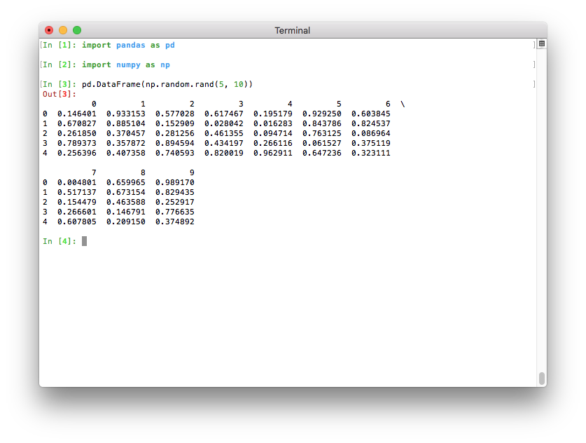
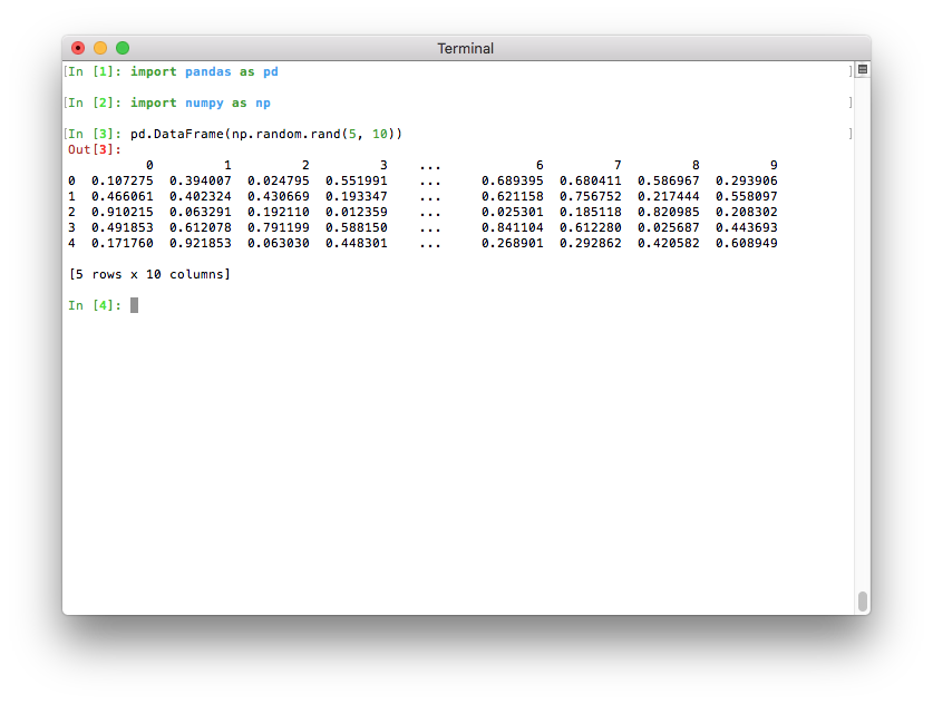
If Python runs in a terminal, the maximum number of columns is now determined automatically so that the printed data frame fits within the current terminal width (pd.options.display.max_columns=0) (GH 17023). If Python runs as a Jupyter kernel (such as the Jupyter QtConsole or a Jupyter notebook, as well as in many IDEs), this value cannot be inferred automatically and is thus set to 20 as in previous versions. In a terminal, this results in a much nicer output:
Note that if you don’t like the new default, you can always set this option yourself. To revert to the old setting, you can run this line:
pd.options.display.max_columns = 20
Datetimelike API changes#
- The default
Timedeltaconstructor now accepts anISO 8601 Durationstring as an argument (GH 19040) - Subtracting
NaTfrom a Series withdtype='datetime64[ns]'returns aSerieswithdtype='timedelta64[ns]'instead ofdtype='datetime64[ns]'(GH 18808) - Addition or subtraction of
NaTfrom TimedeltaIndex will returnTimedeltaIndexinstead ofDatetimeIndex(GH 19124) DatetimeIndex.shift()andTimedeltaIndex.shift()will now raiseNullFrequencyError(which subclassesValueError, which was raised in older versions) when the index object frequency isNone(GH 19147)- Addition and subtraction of
NaNfrom a Series withdtype='timedelta64[ns]'will raise aTypeErrorinstead of treating theNaNasNaT(GH 19274) NaTdivision with datetime.timedelta will now returnNaNinstead of raising (GH 17876)- Operations between a Series with dtype
dtype='datetime64[ns]'and a PeriodIndex will correctly raisesTypeError(GH 18850) - Subtraction of Series with timezone-aware
dtype='datetime64[ns]'with mismatched timezones will raiseTypeErrorinstead ofValueError(GH 18817) - Timestamp will no longer silently ignore unused or invalid
tzortzinfokeyword arguments (GH 17690) - Timestamp will no longer silently ignore invalid
freqarguments (GH 5168) CacheableOffsetandWeekDayare no longer available in thepandas.tseries.offsetsmodule (GH 17830)pandas.tseries.frequencies.get_freq_group()andpandas.tseries.frequencies.DAYSare removed from the public API (GH 18034)- Series.truncate() and DataFrame.truncate() will raise a
ValueErrorif the index is not sorted instead of an unhelpfulKeyError(GH 17935) - Series.first and DataFrame.first will now raise a
TypeErrorrather thanNotImplementedErrorwhen index is not a DatetimeIndex (GH 20725). - Series.last and DataFrame.last will now raise a
TypeErrorrather thanNotImplementedErrorwhen index is not a DatetimeIndex (GH 20725). - Restricted
DateOffsetkeyword arguments. Previously,DateOffsetsubclasses allowed arbitrary keyword arguments which could lead to unexpected behavior. Now, only valid arguments will be accepted. (GH 17176, GH 18226). - pandas.merge() provides a more informative error message when trying to merge on timezone-aware and timezone-naive columns (GH 15800)
- For DatetimeIndex and TimedeltaIndex with
freq=None, addition or subtraction of integer-dtyped array orIndexwill raiseNullFrequencyErrorinstead ofTypeError(GH 19895) - Timestamp constructor now accepts a
nanosecondkeyword or positional argument (GH 18898) - DatetimeIndex will now raise an
AttributeErrorwhen thetzattribute is set after instantiation (GH 3746) - DatetimeIndex with a
pytztimezone will now return a consistentpytztimezone (GH 18595)
Other API changes#
- Series.astype() and Index.astype() with an incompatible dtype will now raise a
TypeErrorrather than aValueError(GH 18231) Seriesconstruction with anobjectdtyped tz-aware datetime anddtype=objectspecified, will now return anobjectdtypedSeries, previously this would infer the datetime dtype (GH 18231)- A Series of
dtype=categoryconstructed from an emptydictwill now have categories ofdtype=objectrather thandtype=float64, consistently with the case in which an empty list is passed (GH 18515) - All-NaN levels in a
MultiIndexare now assignedfloatrather thanobjectdtype, promoting consistency withIndex(GH 17929). - Levels names of a
MultiIndex(when not None) are now required to be unique: trying to create aMultiIndexwith repeated names will raise aValueError(GH 18872) - Both construction and renaming of
Index/MultiIndexwith non-hashablename/nameswill now raiseTypeError(GH 20527) - Index.map() can now accept
Seriesand dictionary input objects (GH 12756, GH 18482, GH 18509). - DataFrame.unstack() will now default to filling with
np.nanforobjectcolumns. (GH 12815) - IntervalIndex constructor will raise if the
closedparameter conflicts with how the input data is inferred to be closed (GH 18421) - Inserting missing values into indexes will work for all types of indexes and automatically insert the correct type of missing value (
NaN,NaT, etc.) regardless of the type passed in (GH 18295) - When created with duplicate labels,
MultiIndexnow raises aValueError. (GH 17464) - Series.fillna() now raises a
TypeErrorinstead of aValueErrorwhen passed a list, tuple or DataFrame as avalue(GH 18293) - pandas.DataFrame.merge() no longer casts a
floatcolumn toobjectwhen merging onintandfloatcolumns (GH 16572) - pandas.merge() now raises a
ValueErrorwhen trying to merge on incompatible data types (GH 9780) - The default NA value for
UInt64Indexhas changed from 0 toNaN, which impacts methods that mask with NA, such asUInt64Index.where()(GH 18398) - Refactored
setup.pyto usefind_packagesinstead of explicitly listing out all subpackages (GH 18535) - Rearranged the order of keyword arguments in read_excel() to align with read_csv() (GH 16672)
- wide_to_long() previously kept numeric-like suffixes as
objectdtype. Now they are cast to numeric if possible (GH 17627) - In read_excel(), the
commentargument is now exposed as a named parameter (GH 18735) - Rearranged the order of keyword arguments in read_excel() to align with read_csv() (GH 16672)
- The options
html.borderandmode.use_inf_as_nullwere deprecated in prior versions, these will now showFutureWarningrather than aDeprecationWarning(GH 19003) - IntervalIndex and
IntervalDtypeno longer support categorical, object, and string subtypes (GH 19016) IntervalDtypenow returnsTruewhen compared against'interval'regardless of subtype, andIntervalDtype.namenow returns'interval'regardless of subtype (GH 18980)KeyErrornow raises instead ofValueErrorin drop(),drop(), drop(), drop() when dropping a non-existent element in an axis with duplicates (GH 19186)- Series.to_csv() now accepts a
compressionargument that works in the same way as thecompressionargument in DataFrame.to_csv() (GH 18958) - Set operations (union, difference…) on IntervalIndex with incompatible index types will now raise a
TypeErrorrather than aValueError(GH 19329) DateOffsetobjects render more simply, e.g.<DateOffset: days=1>instead of<DateOffset: kwds={'days': 1}>(GH 19403)Categorical.fillnanow validates itsvalueandmethodkeyword arguments. It now raises when both or none are specified, matching the behavior of Series.fillna() (GH 19682)pd.to_datetime('today')now returns a datetime, consistent withpd.Timestamp('today'); previouslypd.to_datetime('today')returned a.normalized()datetime (GH 19935)- Series.str.replace() now takes an optional
regexkeyword which, when set toFalse, uses literal string replacement rather than regex replacement (GH 16808) - DatetimeIndex.strftime() and PeriodIndex.strftime() now return an
Indexinstead of a numpy array to be consistent with similar accessors (GH 20127) - Constructing a Series from a list of length 1 no longer broadcasts this list when a longer index is specified (GH 19714, GH 20391).
- DataFrame.to_dict() with
orient='index'no longer casts int columns to float for a DataFrame with only int and float columns (GH 18580) - A user-defined-function that is passed to
Series.rolling().aggregate(),DataFrame.rolling().aggregate(), or its expanding cousins, will now always be passed aSeries, rather than anp.array;.apply()only has therawkeyword, see here. This is consistent with the signatures of.aggregate()across pandas (GH 20584) - Rolling and Expanding types raise
NotImplementedErrorupon iteration (GH 11704).
Deprecations#
Series.from_arrayandSparseSeries.from_arrayare deprecated. Use the normal constructorSeries(..)andSparseSeries(..)instead (GH 18213).DataFrame.as_matrixis deprecated. UseDataFrame.valuesinstead (GH 18458).Series.asobject,DatetimeIndex.asobject,PeriodIndex.asobjectandTimeDeltaIndex.asobjecthave been deprecated. Use.astype(object)instead (GH 18572)- Grouping by a tuple of keys now emits a
FutureWarningand is deprecated. In the future, a tuple passed to'by'will always refer to a single key that is the actual tuple, instead of treating the tuple as multiple keys. To retain the previous behavior, use a list instead of a tuple (GH 18314) Series.validis deprecated. Use Series.dropna() instead (GH 18800).- read_excel() has deprecated the
skip_footerparameter. Useskipfooterinstead (GH 18836) - ExcelFile.parse() has deprecated
sheetnamein favor ofsheet_namefor consistency with read_excel() (GH 20920). - The
is_copyattribute is deprecated and will be removed in a future version (GH 18801). IntervalIndex.from_intervalsis deprecated in favor of the IntervalIndex constructor (GH 19263)DataFrame.from_itemsis deprecated. Use DataFrame.from_dict() instead, orDataFrame.from_dict(OrderedDict())if you wish to preserve the key order (GH 17320, GH 17312)- Indexing a MultiIndex or a
FloatIndexwith a list containing some missing keys will now show a FutureWarning, which is consistent with other types of indexes (GH 17758). - The
broadcastparameter of.apply()is deprecated in favor ofresult_type='broadcast'(GH 18577) - The
reduceparameter of.apply()is deprecated in favor ofresult_type='reduce'(GH 18577) - The
orderparameter of factorize() is deprecated and will be removed in a future release (GH 19727) Timestamp.weekday_name,DatetimeIndex.weekday_name, andSeries.dt.weekday_nameare deprecated in favor of Timestamp.day_name(), DatetimeIndex.day_name(), and Series.dt.day_name() (GH 12806)pandas.tseries.plotting.tsplotis deprecated. Use Series.plot() instead (GH 18627)Index.summary()is deprecated and will be removed in a future version (GH 18217)NDFrame.get_ftype_counts()is deprecated and will be removed in a future version (GH 18243)- The
convert_datetime64parameter in DataFrame.to_records() has been deprecated and will be removed in a future version. The NumPy bug motivating this parameter has been resolved. The default value for this parameter has also changed fromTruetoNone(GH 18160). Series.rolling().apply(),DataFrame.rolling().apply(),Series.expanding().apply(), andDataFrame.expanding().apply()have deprecated passing annp.arrayby default. One will need to pass the newrawparameter to be explicit about what is passed (GH 20584)- The
data,base,strides,flagsanditemsizeproperties of theSeriesandIndexclasses have been deprecated and will be removed in a future version (GH 20419). DatetimeIndex.offsetis deprecated. UseDatetimeIndex.freqinstead (GH 20716)- Floor division between an integer ndarray and a Timedelta is deprecated. Divide by Timedelta.value instead (GH 19761)
- Setting
PeriodIndex.freq(which was not guaranteed to work correctly) is deprecated. Use PeriodIndex.asfreq() instead (GH 20678) Index.get_duplicates()is deprecated and will be removed in a future version (GH 20239)- The previous default behavior of negative indices in
Categorical.takeis deprecated. In a future version it will change from meaning missing values to meaning positional indices from the right. The future behavior is consistent with Series.take() (GH 20664). - Passing multiple axes to the
axisparameter in DataFrame.dropna() has been deprecated and will be removed in a future version (GH 20987)
Removal of prior version deprecations/changes#
- Warnings against the obsolete usage
Categorical(codes, categories), which were emitted for instance when the first two arguments toCategorical()had different dtypes, and recommended the use ofCategorical.from_codes, have now been removed (GH 8074) - The
levelsandlabelsattributes of aMultiIndexcan no longer be set directly (GH 4039). pd.tseries.util.pivot_annualhas been removed (deprecated since v0.19). Usepivot_tableinstead (GH 18370)pd.tseries.util.isleapyearhas been removed (deprecated since v0.19). Use.is_leap_yearproperty in Datetime-likes instead (GH 18370)pd.ordered_mergehas been removed (deprecated since v0.19). Usepd.merge_orderedinstead (GH 18459)- The
SparseListclass has been removed (GH 14007) - The
pandas.io.wbandpandas.io.datastub modules have been removed (GH 13735) Categorical.from_arrayhas been removed (GH 13854)- The
freqandhowparameters have been removed from therolling/expanding/ewmmethods of DataFrame and Series (deprecated since v0.18). Instead, resample before calling the methods. (GH 18601 & GH 18668) DatetimeIndex.to_datetime,Timestamp.to_datetime,PeriodIndex.to_datetime, andIndex.to_datetimehave been removed (GH 8254, GH 14096, GH 14113)- read_csv() has dropped the
skip_footerparameter (GH 13386) - read_csv() has dropped the
as_recarrayparameter (GH 13373) - read_csv() has dropped the
buffer_linesparameter (GH 13360) - read_csv() has dropped the
compact_intsanduse_unsignedparameters (GH 13323) - The
Timestampclass has dropped theoffsetattribute in favor offreq(GH 13593) - The
Series,Categorical, andIndexclasses have dropped thereshapemethod (GH 13012) pandas.tseries.frequencies.get_standard_freqhas been removed in favor ofpandas.tseries.frequencies.to_offset(freq).rule_code(GH 13874)- The
freqstrkeyword has been removed frompandas.tseries.frequencies.to_offsetin favor offreq(GH 13874) - The
Panel4DandPanelNDclasses have been removed (GH 13776) - The
Panelclass has dropped theto_longandtoLongmethods (GH 19077) - The options
display.line_withanddisplay.heightare removed in favor ofdisplay.widthanddisplay.max_rowsrespectively (GH 4391, GH 19107) - The
labelsattribute of theCategoricalclass has been removed in favor of Categorical.codes (GH 7768) - The
flavorparameter have been removed fromto_sql()method (GH 13611) - The modules
pandas.tools.hashingandpandas.util.hashinghave been removed (GH 16223) - The top-level functions
pd.rolling_*,pd.expanding_*andpd.ewm*have been removed (Deprecated since v0.18). Instead, use the DataFrame/Series methods rolling, expanding and ewm (GH 18723) - Imports from
pandas.core.commonfor functions such asis_datetime64_dtypeare now removed. These are located inpandas.api.types. (GH 13634, GH 19769) - The
infer_dstkeyword in Series.tz_localize(), DatetimeIndex.tz_localize()and DatetimeIndex have been removed.infer_dst=Trueis equivalent toambiguous='infer', andinfer_dst=Falsetoambiguous='raise'(GH 7963). - When
.resample()was changed from an eager to a lazy operation, like.groupby()in v0.18.0, we put in place compatibility (with aFutureWarning), so operations would continue to work. This is now fully removed, so aResamplerwill no longer forward compat operations (GH 20554) - Remove long deprecated
axis=Noneparameter from.replace()(GH 20271)
Performance improvements#
- Indexers on
SeriesorDataFrameno longer create a reference cycle (GH 17956) - Added a keyword argument,
cache, to to_datetime() that improved the performance of converting duplicate datetime arguments (GH 11665) DateOffsetarithmetic performance is improved (GH 18218)- Converting a
SeriesofTimedeltaobjects to days, seconds, etc… sped up through vectorization of underlying methods (GH 18092) - Improved performance of
.map()with aSeries/dictinput (GH 15081) - The overridden
Timedeltaproperties of days, seconds and microseconds have been removed, leveraging their built-in Python versions instead (GH 18242) Seriesconstruction will reduce the number of copies made of the input data in certain cases (GH 17449)- Improved performance of Series.dt.date() and DatetimeIndex.date() (GH 18058)
- Improved performance of Series.dt.time() and DatetimeIndex.time() (GH 18461)
- Improved performance of
IntervalIndex.symmetric_difference()(GH 18475) - Improved performance of
DatetimeIndexandSeriesarithmetic operations with Business-Month and Business-Quarter frequencies (GH 18489) - Series() / DataFrame() tab completion limits to 100 values, for better performance. (GH 18587)
- Improved performance of DataFrame.median() with
axis=1when bottleneck is not installed (GH 16468) - Improved performance of MultiIndex.get_loc() for large indexes, at the cost of a reduction in performance for small ones (GH 18519)
- Improved performance of MultiIndex.remove_unused_levels() when there are no unused levels, at the cost of a reduction in performance when there are (GH 19289)
- Improved performance of Index.get_loc() for non-unique indexes (GH 19478)
- Improved performance of pairwise
.rolling()and.expanding()with.cov()and.corr()operations (GH 17917) - Improved performance of
GroupBy.rank()(GH 15779) - Improved performance of variable
.rolling()on.min()and.max()(GH 19521) - Improved performance of
GroupBy.ffill()andGroupBy.bfill()(GH 11296) - Improved performance of
GroupBy.any()andGroupBy.all()(GH 15435) - Improved performance of
GroupBy.pct_change()(GH 19165) - Improved performance of Series.isin() in the case of categorical dtypes (GH 20003)
- Improved performance of
getattr(Series, attr)when the Series has certain index types. This manifested in slow printing of large Series with aDatetimeIndex(GH 19764) - Fixed a performance regression for
GroupBy.nth()andGroupBy.last()with some object columns (GH 19283) - Improved performance of
Categorical.from_codes()(GH 18501)
Documentation changes#
Thanks to all of the contributors who participated in the pandas Documentation Sprint, which took place on March 10th. We had about 500 participants from over 30 locations across the world. You should notice that many of theAPI docstrings have greatly improved.
There were too many simultaneous contributions to include a release note for each improvement, but this GitHub search should give you an idea of how many docstrings were improved.
Special thanks to Marc Garcia for organizing the sprint. For more information, read the NumFOCUS blogpost recapping the sprint.
- Changed spelling of “numpy” to “NumPy”, and “python” to “Python”. (GH 19017)
- Consistency when introducing code samples, using either colon or period. Rewrote some sentences for greater clarity, added more dynamic references to functions, methods and classes. (GH 18941, GH 18948, GH 18973, GH 19017)
- Added a reference to DataFrame.assign() in the concatenate section of the merging documentation (GH 18665)
Bug fixes#
Categorical#
Warning
A class of bugs were introduced in pandas 0.21 with CategoricalDtype that affects the correctness of operations like merge, concat, and indexing when comparing multiple unordered Categorical arrays that have the same categories, but in a different order. We highly recommend upgrading or manually aligning your categories before doing these operations.
- Bug in
Categorical.equalsreturning the wrong result when comparing two unorderedCategoricalarrays with the same categories, but in a different order (GH 16603) - Bug in pandas.api.types.union_categoricals() returning the wrong result when for unordered categoricals with the categories in a different order. This affected pandas.concat() with Categorical data (GH 19096).
- Bug in pandas.merge() returning the wrong result when joining on an unordered
Categoricalthat had the same categories but in a different order (GH 19551) - Bug in
CategoricalIndex.get_indexer()returning the wrong result whentargetwas an unorderedCategoricalthat had the same categories asselfbut in a different order (GH 19551) - Bug in Index.astype() with a categorical dtype where the resultant index is not converted to a CategoricalIndex for all types of index (GH 18630)
- Bug in Series.astype() and
Categorical.astype()where an existing categorical data does not get updated (GH 10696, GH 18593) - Bug in Series.str.split() with
expand=Trueincorrectly raising an IndexError on empty strings (GH 20002). - Bug in Index constructor with
dtype=CategoricalDtype(...)wherecategoriesandorderedare not maintained (GH 19032) - Bug in Series constructor with scalar and
dtype=CategoricalDtype(...)wherecategoriesandorderedare not maintained (GH 19565) - Bug in
Categorical.__iter__not converting to Python types (GH 19909) - Bug in pandas.factorize() returning the unique codes for the
uniques. This now returns aCategoricalwith the same dtype as the input (GH 19721) - Bug in pandas.factorize() including an item for missing values in the
uniquesreturn value (GH 19721) - Bug in Series.take() with categorical data interpreting
-1inindicesas missing value markers, rather than the last element of the Series (GH 20664)
Datetimelike#
- Bug in
Series.__sub__()subtracting a non-nanosecondnp.datetime64object from aSeriesgave incorrect results (GH 7996) - Bug in DatetimeIndex, TimedeltaIndex addition and subtraction of zero-dimensional integer arrays gave incorrect results (GH 19012)
- Bug in DatetimeIndex and TimedeltaIndex where adding or subtracting an array-like of
DateOffsetobjects either raised (np.array,pd.Index) or broadcast incorrectly (pd.Series) (GH 18849) - Bug in
Series.__add__()adding Series with dtypetimedelta64[ns]to a timezone-awareDatetimeIndexincorrectly dropped timezone information (GH 13905) - Adding a
Periodobject to adatetimeorTimestampobject will now correctly raise aTypeError(GH 17983) - Bug in Timestamp where comparison with an array of
Timestampobjects would result in aRecursionError(GH 15183) - Bug in Series floor-division where operating on a scalar
timedeltaraises an exception (GH 18846) - Bug in DatetimeIndex where the repr was not showing high-precision time values at the end of a day (e.g., 23:59:59.999999999) (GH 19030)
- Bug in
.astype()to non-ns timedelta units would hold the incorrect dtype (GH 19176, GH 19223, GH 12425) - Bug in subtracting Series from
NaTincorrectly returningNaT(GH 19158) - Bug in Series.truncate() which raises
TypeErrorwith a monotonicPeriodIndex(GH 17717) - Bug in pct_change() using
periodsandfreqreturned different length outputs (GH 7292) - Bug in comparison of DatetimeIndex against
Noneordatetime.dateobjects raisingTypeErrorfor==and!=comparisons instead of all-Falseand all-True, respectively (GH 19301) - Bug in Timestamp and to_datetime() where a string representing a barely out-of-bounds timestamp would be incorrectly rounded down instead of raising
OutOfBoundsDatetime(GH 19382) - Bug in Timestamp.floor() DatetimeIndex.floor() where time stamps far in the future and past were not rounded correctly (GH 19206)
- Bug in to_datetime() where passing an out-of-bounds datetime with
errors='coerce'andutc=Truewould raiseOutOfBoundsDatetimeinstead of parsing toNaT(GH 19612) - Bug in DatetimeIndex and TimedeltaIndex addition and subtraction where name of the returned object was not always set consistently. (GH 19744)
- Bug in DatetimeIndex and TimedeltaIndex addition and subtraction where operations with numpy arrays raised
TypeError(GH 19847) - Bug in DatetimeIndex and TimedeltaIndex where setting the
freqattribute was not fully supported (GH 20678)
Timedelta#
- Bug in
Timedelta.__mul__()where multiplying byNaTreturnedNaTinstead of raising aTypeError(GH 19819) - Bug in Series with
dtype='timedelta64[ns]'where addition or subtraction ofTimedeltaIndexhad results cast todtype='int64'(GH 17250) - Bug in Series with
dtype='timedelta64[ns]'where addition or subtraction ofTimedeltaIndexcould return aSerieswith an incorrect name (GH 19043) - Bug in
Timedelta.__floordiv__()andTimedelta.__rfloordiv__()dividing by many incompatible numpy objects was incorrectly allowed (GH 18846) - Bug where dividing a scalar timedelta-like object with TimedeltaIndex performed the reciprocal operation (GH 19125)
- Bug in TimedeltaIndex where division by a
Serieswould return aTimedeltaIndexinstead of aSeries(GH 19042) - Bug in
Timedelta.__add__(),Timedelta.__sub__()where adding or subtracting anp.timedelta64object would return anothernp.timedelta64instead of aTimedelta(GH 19738) - Bug in
Timedelta.__floordiv__(),Timedelta.__rfloordiv__()where operating with aTickobject would raise aTypeErrorinstead of returning a numeric value (GH 19738) - Bug in Period.asfreq() where periods near
datetime(1, 1, 1)could be converted incorrectly (GH 19643, GH 19834) - Bug in Timedelta.total_seconds() causing precision errors, for example
Timedelta('30S').total_seconds()==30.000000000000004(GH 19458) - Bug in
Timedelta.__rmod__()where operating with anumpy.timedelta64returned atimedelta64object instead of aTimedelta(GH 19820) - Multiplication of TimedeltaIndex by
TimedeltaIndexwill now raiseTypeErrorinstead of raisingValueErrorin cases of length mismatch (GH 19333) - Bug in indexing a TimedeltaIndex with a
np.timedelta64object which was raising aTypeError(GH 20393)
Timezones#
- Bug in creating a
Seriesfrom an array that contains both tz-naive and tz-aware values will result in aSerieswhose dtype is tz-aware instead of object (GH 16406) - Bug in comparison of timezone-aware DatetimeIndex against
NaTincorrectly raisingTypeError(GH 19276) - Bug in
DatetimeIndex.astype()when converting between timezone aware dtypes, and converting from timezone aware to naive (GH 18951) - Bug in comparing DatetimeIndex, which failed to raise
TypeErrorwhen attempting to compare timezone-aware and timezone-naive datetimelike objects (GH 18162) - Bug in localization of a naive, datetime string in a
Seriesconstructor with adatetime64[ns, tz]dtype (GH 174151) - Timestamp.replace() will now handle Daylight Savings transitions gracefully (GH 18319)
- Bug in tz-aware DatetimeIndex where addition/subtraction with a TimedeltaIndex or array with
dtype='timedelta64[ns]'was incorrect (GH 17558) - Bug in
DatetimeIndex.insert()where insertingNaTinto a timezone-aware index incorrectly raised (GH 16357) - Bug in DataFrame constructor, where tz-aware Datetimeindex and a given column name will result in an empty
DataFrame(GH 19157) - Bug in Timestamp.tz_localize() where localizing a timestamp near the minimum or maximum valid values could overflow and return a timestamp with an incorrect nanosecond value (GH 12677)
- Bug when iterating over DatetimeIndex that was localized with fixed timezone offset that rounded nanosecond precision to microseconds (GH 19603)
- Bug in DataFrame.diff() that raised an
IndexErrorwith tz-aware values (GH 18578) - Bug in melt() that converted tz-aware dtypes to tz-naive (GH 15785)
- Bug in
Dataframe.count()that raised anValueError, ifDataframe.dropna()was called for a single column with timezone-aware values. (GH 13407)
Offsets#
- Bug in
WeekOfMonthandWeekwhere addition and subtraction did not roll correctly (GH 18510, GH 18672, GH 18864) - Bug in
WeekOfMonthandLastWeekOfMonthwhere default keyword arguments for constructor raisedValueError(GH 19142) - Bug in
FY5253Quarter,LastWeekOfMonthwhere rollback and rollforward behavior was inconsistent with addition and subtraction behavior (GH 18854) - Bug in
FY5253wheredatetimeaddition and subtraction incremented incorrectly for dates on the year-end but not normalized to midnight (GH 18854) - Bug in
FY5253where date offsets could incorrectly raise anAssertionErrorin arithmetic operations (GH 14774)
Numeric#
- Bug in Series constructor with an int or float list where specifying
dtype=str,dtype='str'ordtype='U'failed to convert the data elements to strings (GH 16605) - Bug in Index multiplication and division methods where operating with a
Serieswould return anIndexobject instead of aSeriesobject (GH 19042) - Bug in the DataFrame constructor in which data containing very large positive or very large negative numbers was causing
OverflowError(GH 18584) - Bug in Index constructor with
dtype='uint64'where int-like floats were not coerced toUInt64Index(GH 18400) - Bug in DataFrame flex arithmetic (e.g.
df.add(other, fill_value=foo)) with afill_valueother thanNonefailed to raiseNotImplementedErrorin corner cases where either the frame orotherhas length zero (GH 19522) - Multiplication and division of numeric-dtyped Index objects with timedelta-like scalars returns
TimedeltaIndexinstead of raisingTypeError(GH 19333) - Bug where
NaNwas returned instead of 0 by Series.pct_change() and DataFrame.pct_change() whenfill_methodis notNone(GH 19873)
Strings#
- Bug in Series.str.get() with a dictionary in the values and the index not in the keys, raising
KeyError(GH 20671)
Indexing#
- Bug in Index construction from list of mixed type tuples (GH 18505)
- Bug in Index.drop() when passing a list of both tuples and non-tuples (GH 18304)
- Bug in DataFrame.drop(),
Panel.drop(), Series.drop(), Index.drop() where noKeyErroris raised when dropping a non-existent element from an axis that contains duplicates (GH 19186) - Bug in indexing a datetimelike
Indexthat raisedValueErrorinstead ofIndexError(GH 18386). - Index.to_series() now accepts
indexandnamekwargs (GH 18699) - DatetimeIndex.to_series() now accepts
indexandnamekwargs (GH 18699) - Bug in indexing non-scalar value from
Serieshaving non-uniqueIndexwill return value flattened (GH 17610) - Bug in indexing with iterator containing only missing keys, which raised no error (GH 20748)
- Fixed inconsistency in
.ixbetween list and scalar keys when the index has integer dtype and does not include the desired keys (GH 20753) - Bug in
__setitem__when indexing a DataFrame with a 2-d boolean ndarray (GH 18582) - Bug in
str.extractallwhen there were no matches empty Index was returned instead of appropriate MultiIndex (GH 19034) - Bug in IntervalIndex where empty and purely NA data was constructed inconsistently depending on the construction method (GH 18421)
- Bug in
IntervalIndex.symmetric_difference()where the symmetric difference with a non-IntervalIndexdid not raise (GH 18475) - Bug in IntervalIndex where set operations that returned an empty
IntervalIndexhad the wrong dtype (GH 19101) - Bug in DataFrame.drop_duplicates() where no
KeyErroris raised when passing in columns that don’t exist on theDataFrame(GH 19726) - Bug in
Indexsubclasses constructors that ignore unexpected keyword arguments (GH 19348) - Bug in Index.difference() when taking difference of an
Indexwith itself (GH 20040) - Bug in DataFrame.first_valid_index() and DataFrame.last_valid_index() in presence of entire rows of NaNs in the middle of values (GH 20499).
- Bug in IntervalIndex where some indexing operations were not supported for overlapping or non-monotonic
uint64data (GH 20636) - Bug in
Series.is_uniquewhere extraneous output in stderr is shown if Series contains objects with__ne__defined (GH 20661) - Bug in
.locassignment with a single-element list-like incorrectly assigns as a list (GH 19474) - Bug in partial string indexing on a
Series/DataFramewith a monotonic decreasingDatetimeIndex(GH 19362) - Bug in performing in-place operations on a
DataFramewith a duplicateIndex(GH 17105) - Bug in IntervalIndex.get_loc() and IntervalIndex.get_indexer() when used with an IntervalIndex containing a single interval (GH 17284, GH 20921)
- Bug in
.locwith auint64indexer (GH 20722)
MultiIndex#
- Bug in
MultiIndex.__contains__()where non-tuple keys would returnTrueeven if they had been dropped (GH 19027) - Bug in
MultiIndex.set_labels()which would cause casting (and potentially clipping) of the new labels if thelevelargument is not 0 or a list like [0, 1, … ] (GH 19057) - Bug in MultiIndex.get_level_values() which would return an invalid index on level of ints with missing values (GH 17924)
- Bug in
MultiIndex.unique()when called on empty MultiIndex (GH 20568) - Bug in
MultiIndex.unique()which would not preserve level names (GH 20570) - Bug in MultiIndex.remove_unused_levels() which would fill nan values (GH 18417)
- Bug in MultiIndex.from_tuples() which would fail to take zipped tuples in python3 (GH 18434)
- Bug in MultiIndex.get_loc() which would fail to automatically cast values between float and int (GH 18818, GH 15994)
- Bug in MultiIndex.get_loc() which would cast boolean to integer labels (GH 19086)
- Bug in MultiIndex.get_loc() which would fail to locate keys containing
NaN(GH 18485) - Bug in MultiIndex.get_loc() in large MultiIndex, would fail when levels had different dtypes (GH 18520)
- Bug in indexing where nested indexers having only numpy arrays are handled incorrectly (GH 19686)
IO#
- read_html() now rewinds seekable IO objects after parse failure, before attempting to parse with a new parser. If a parser errors and the object is non-seekable, an informative error is raised suggesting the use of a different parser (GH 17975)
- DataFrame.to_html() now has an option to add an id to the leading
<table>tag (GH 8496) - Bug in
read_msgpack()with a non existent file is passed in Python 2 (GH 15296) - Bug in read_csv() where a
MultiIndexwith duplicate columns was not being mangled appropriately (GH 18062) - Bug in read_csv() where missing values were not being handled properly when
keep_default_na=Falsewith dictionaryna_values(GH 19227) - Bug in read_csv() causing heap corruption on 32-bit, big-endian architectures (GH 20785)
- Bug in read_sas() where a file with 0 variables gave an
AttributeErrorincorrectly. Now it gives anEmptyDataError(GH 18184) - Bug in DataFrame.to_latex() where pairs of braces meant to serve as invisible placeholders were escaped (GH 18667)
- Bug in DataFrame.to_latex() where a
NaNin aMultiIndexwould cause anIndexErroror incorrect output (GH 14249) - Bug in DataFrame.to_latex() where a non-string index-level name would result in an
AttributeError(GH 19981) - Bug in DataFrame.to_latex() where the combination of an index name and the
index_names=Falseoption would result in incorrect output (GH 18326) - Bug in DataFrame.to_latex() where a
MultiIndexwith an empty string as its name would result in incorrect output (GH 18669) - Bug in DataFrame.to_latex() where missing space characters caused wrong escaping and produced non-valid latex in some cases (GH 20859)
- Bug in read_json() where large numeric values were causing an
OverflowError(GH 18842) - Bug in DataFrame.to_parquet() where an exception was raised if the write destination is S3 (GH 19134)
- Interval now supported in DataFrame.to_excel() for all Excel file types (GH 19242)
- Timedelta now supported in DataFrame.to_excel() for all Excel file types (GH 19242, GH 9155, GH 19900)
- Bug in pandas.io.stata.StataReader.value_labels() raising an
AttributeErrorwhen called on very old files. Now returns an empty dict (GH 19417) - Bug in read_pickle() when unpickling objects with TimedeltaIndex or
Float64Indexcreated with pandas prior to version 0.20 (GH 19939) - Bug in
pandas.io.json.json_normalize()where sub-records are not properly normalized if any sub-records values are NoneType (GH 20030) - Bug in
usecolsparameter in read_csv() where error is not raised correctly when passing a string. (GH 20529) - Bug in HDFStore.keys() when reading a file with a soft link causes exception (GH 20523)
- Bug in
HDFStore.select_column()where a key which is not a valid store raised anAttributeErrorinstead of aKeyError(GH 17912)
Plotting#
- Better error message when attempting to plot but matplotlib is not installed (GH 19810).
- DataFrame.plot() now raises a
ValueErrorwhen thexoryargument is improperly formed (GH 18671) - Bug in DataFrame.plot() when
xandyarguments given as positions caused incorrect referenced columns for line, bar and area plots (GH 20056) - Bug in formatting tick labels with
datetime.time()and fractional seconds (GH 18478). - Series.plot.kde() has exposed the args
indandbw_methodin the docstring (GH 18461). The argumentindmay now also be an integer (number of sample points). - DataFrame.plot() now supports multiple columns to the
yargument (GH 19699)
GroupBy/resample/rolling#
- Bug when grouping by a single column and aggregating with a class like
listortuple(GH 18079) - Fixed regression in DataFrame.groupby() which would not emit an error when called with a tuple key not in the index (GH 18798)
- Bug in DataFrame.resample() which silently ignored unsupported (or mistyped) options for
label,closedandconvention(GH 19303) - Bug in DataFrame.groupby() where tuples were interpreted as lists of keys rather than as keys (GH 17979, GH 18249)
- Bug in DataFrame.groupby() where aggregation by
first/last/min/maxwas causing timestamps to lose precision (GH 19526) - Bug in DataFrame.transform() where particular aggregation functions were being incorrectly cast to match the dtype(s) of the grouped data (GH 19200)
- Bug in DataFrame.groupby() passing the
on=kwarg, and subsequently using.apply()(GH 17813) - Bug in
DataFrame.resample().aggregatenot raising aKeyErrorwhen aggregating a non-existent column (GH 16766, GH 19566) - Bug in
DataFrameGroupBy.cumsum()andDataFrameGroupBy.cumprod()whenskipnawas passed (GH 19806) - Bug in DataFrame.resample() that dropped timezone information (GH 13238)
- Bug in DataFrame.groupby() where transformations using
np.allandnp.anywere raising aValueError(GH 20653) - Bug in DataFrame.resample() where
ffill,bfill,pad,backfill,fillna,interpolate, andasfreqwere ignoringloffset. (GH 20744) - Bug in DataFrame.groupby() when applying a function that has mixed data types and the user supplied function can fail on the grouping column (GH 20949)
- Bug in
DataFrameGroupBy.rolling().apply()where operations performed against the associatedDataFrameGroupByobject could impact the inclusion of the grouped item(s) in the result (GH 14013)
Sparse#
- Bug in which creating a
SparseDataFramefrom a denseSeriesor an unsupported type raised an uncontrolled exception (GH 19374) - Bug in
SparseDataFrame.to_csvcausing exception (GH 19384) - Bug in
SparseSeries.memory_usagewhich caused segfault by accessing non sparse elements (GH 19368) - Bug in constructing a
SparseArray: ifdatais a scalar andindexis defined it will coerce tofloat64regardless of scalar’s dtype. (GH 19163)
Reshaping#
- Bug in DataFrame.merge() where referencing a
CategoricalIndexby name, where thebykwarg wouldKeyError(GH 20777) - Bug in DataFrame.stack() which fails trying to sort mixed type levels under Python 3 (GH 18310)
- Bug in DataFrame.unstack() which casts int to float if
columnsis aMultiIndexwith unused levels (GH 17845) - Bug in DataFrame.unstack() which raises an error if
indexis aMultiIndexwith unused labels on the unstacked level (GH 18562) - Fixed construction of a Series from a
dictcontainingNaNas key (GH 18480) - Fixed construction of a DataFrame from a
dictcontainingNaNas key (GH 18455) - Disabled construction of a Series where len(index) > len(data) = 1, which previously would broadcast the data item, and now raises a
ValueError(GH 18819) - Suppressed error in the construction of a DataFrame from a
dictcontaining scalar values when the corresponding keys are not included in the passed index (GH 18600) - Fixed (changed from
objecttofloat64) dtype of DataFrame initialized with axes, no data, anddtype=int(GH 19646) - Bug in Series.rank() where
SeriescontainingNaTmodifies theSeriesinplace (GH 18521) - Bug in cut() which fails when using readonly arrays (GH 18773)
- Bug in DataFrame.pivot_table() which fails when the
aggfuncarg is of type string. The behavior is now consistent with other methods likeaggandapply(GH 18713) - Bug in DataFrame.merge() in which merging using
Indexobjects as vectors raised an Exception (GH 19038) - Bug in DataFrame.stack(), DataFrame.unstack(), Series.unstack() which were not returning subclasses (GH 15563)
- Bug in timezone comparisons, manifesting as a conversion of the index to UTC in
.concat()(GH 18523) - Bug in concat() when concatenating sparse and dense series it returns only a
SparseDataFrame. Should be aDataFrame. (GH 18914, GH 18686, and GH 16874) - Improved error message for DataFrame.merge() when there is no common merge key (GH 19427)
- Bug in DataFrame.join() which does an
outerinstead of aleftjoin when being called with multiple DataFrames and some have non-unique indices (GH 19624) - Series.rename() now accepts
axisas a kwarg (GH 18589) - Bug in rename() where an Index of same-length tuples was converted to a MultiIndex (GH 19497)
- Comparisons between Series and Index would return a
Serieswith an incorrect name, ignoring theIndex’s name attribute (GH 19582) - Bug in qcut() where datetime and timedelta data with
NaTpresent raised aValueError(GH 19768) - Bug in DataFrame.iterrows(), which would infers strings not compliant to ISO8601 to datetimes (GH 19671)
- Bug in Series constructor with
Categoricalwhere aValueErroris not raised when an index of different length is given (GH 19342) - Bug in DataFrame.astype() where column metadata is lost when converting to categorical or a dictionary of dtypes (GH 19920)
- Bug in cut() and qcut() where timezone information was dropped (GH 19872)
- Bug in Series constructor with a
dtype=str, previously raised in some cases (GH 19853) - Bug in get_dummies(), and
select_dtypes(), where duplicate column names caused incorrect behavior (GH 20848) - Bug in isna(), which cannot handle ambiguous typed lists (GH 20675)
- Bug in concat() which raises an error when concatenating TZ-aware dataframes and all-NaT dataframes (GH 12396)
- Bug in concat() which raises an error when concatenating empty TZ-aware series (GH 18447)
Other#
- Improved error message when attempting to use a Python keyword as an identifier in a
numexprbacked query (GH 18221) - Bug in accessing a pandas.get_option(), which raised
KeyErrorrather thanOptionErrorwhen looking up a non-existent option key in some cases (GH 19789) - Bug in testing.assert_series_equal() and testing.assert_frame_equal() for Series or DataFrames with differing unicode data (GH 20503)
Contributors#
A total of 328 people contributed patches to this release. People with a “+” by their names contributed a patch for the first time.
- Aaron Critchley
- AbdealiJK +
- Adam Hooper +
- Albert Villanova del Moral
- Alejandro Giacometti +
- Alejandro Hohmann +
- Alex Rychyk
- Alexander Buchkovsky
- Alexander Lenail +
- Alexander Michael Schade
- Aly Sivji +
- Andreas Költringer +
- Andrew
- Andrew Bui +
- András Novoszáth +
- Andy Craze +
- Andy R. Terrel
- Anh Le +
- Anil Kumar Pallekonda +
- Antoine Pitrou +
- Antonio Linde +
- Antonio Molina +
- Antonio Quinonez +
- Armin Varshokar +
- Artem Bogachev +
- Avi Sen +
- Azeez Oluwafemi +
- Ben Auffarth +
- Bernhard Thiel +
- Bhavesh Poddar +
- BielStela +
- Blair +
- Bob Haffner
- Brett Naul +
- Brock Mendel
- Bryce Guinta +
- Carlos Eduardo Moreira dos Santos +
- Carlos García Márquez +
- Carol Willing
- Cheuk Ting Ho +
- Chitrank Dixit +
- Chris
- Chris Burr +
- Chris Catalfo +
- Chris Mazzullo
- Christian Chwala +
- Cihan Ceyhan +
- Clemens Brunner
- Colin +
- Cornelius Riemenschneider
- Crystal Gong +
- DaanVanHauwermeiren
- Dan Dixey +
- Daniel Frank +
- Daniel Garrido +
- Daniel Sakuma +
- DataOmbudsman +
- Dave Hirschfeld
- Dave Lewis +
- David Adrián Cañones Castellano +
- David Arcos +
- David C Hall +
- David Fischer
- David Hoese +
- David Lutz +
- David Polo +
- David Stansby
- Dennis Kamau +
- Dillon Niederhut
- Dimitri +
- Dr. Irv
- Dror Atariah
- Eric Chea +
- Eric Kisslinger
- Eric O. LEBIGOT (EOL) +
- FAN-GOD +
- Fabian Retkowski +
- Fer Sar +
- Gabriel de Maeztu +
- Gianpaolo Macario +
- Giftlin Rajaiah
- Gilberto Olimpio +
- Gina +
- Gjelt +
- Graham Inggs +
- Grant Roch
- Grant Smith +
- Grzegorz Konefał +
- Guilherme Beltramini
- HagaiHargil +
- Hamish Pitkeathly +
- Hammad Mashkoor +
- Hannah Ferchland +
- Hans
- Haochen Wu +
- Hissashi Rocha +
- Iain Barr +
- Ibrahim Sharaf ElDen +
- Ignasi Fosch +
- Igor Conrado Alves de Lima +
- Igor Shelvinskyi +
- Imanflow +
- Ingolf Becker
- Israel Saeta Pérez
- Iva Koevska +
- Jakub Nowacki +
- Jan F-F +
- Jan Koch +
- Jan Werkmann
- Janelle Zoutkamp +
- Jason Bandlow +
- Jaume Bonet +
- Jay Alammar +
- Jeff Reback
- JennaVergeynst
- Jimmy Woo +
- Jing Qiang Goh +
- Joachim Wagner +
- Joan Martin Miralles +
- Joel Nothman
- Joeun Park +
- John Cant +
- Johnny Metz +
- Jon Mease
- Jonas Schulze +
- Jongwony +
- Jordi Contestí +
- Joris Van den Bossche
- José F. R. Fonseca +
- Jovixe +
- Julio Martinez +
- Jörg Döpfert
- KOBAYASHI Ittoku +
- Kate Surta +
- Kenneth +
- Kevin Kuhl
- Kevin Sheppard
- Krzysztof Chomski
- Ksenia +
- Ksenia Bobrova +
- Kunal Gosar +
- Kurtis Kerstein +
- Kyle Barron +
- Laksh Arora +
- Laurens Geffert +
- Leif Walsh
- Liam Marshall +
- Liam3851 +
- Licht Takeuchi
- Liudmila +
- Ludovico Russo +
- Mabel Villalba +
- Manan Pal Singh +
- Manraj Singh
- Marc +
- Marc Garcia
- Marco Hemken +
- Maria del Mar Bibiloni +
- Mario Corchero +
- Mark Woodbridge +
- Martin Journois +
- Mason Gallo +
- Matias Heikkilä +
- Matt Braymer-Hayes
- Matt Kirk +
- Matt Maybeno +
- Matthew Kirk +
- Matthew Rocklin +
- Matthew Roeschke
- Matthias Bussonnier +
- Max Mikhaylov +
- Maxim Veksler +
- Maximilian Roos
- Maximiliano Greco +
- Michael Penkov
- Michael Röttger +
- Michael Selik +
- Michael Waskom
- Mie~~~
- Mike Kutzma +
- Ming Li +
- Mitar +
- Mitch Negus +
- Montana Low +
- Moritz Münst +
- Mortada Mehyar
- Myles Braithwaite +
- Nate Yoder
- Nicholas Ursa +
- Nick Chmura
- Nikos Karagiannakis +
- Nipun Sadvilkar +
- Nis Martensen +
- Noah +
- Noémi Éltető +
- Olivier Bilodeau +
- Ondrej Kokes +
- Onno Eberhard +
- Paul Ganssle +
- Paul Mannino +
- Paul Reidy
- Paulo Roberto de Oliveira Castro +
- Pepe Flores +
- Peter Hoffmann
- Phil Ngo +
- Pietro Battiston
- Pranav Suri +
- Priyanka Ojha +
- Pulkit Maloo +
- README Bot +
- Ray Bell +
- Riccardo Magliocchetti +
- Ridhwan Luthra +
- Robert Meyer
- Robin
- Robin Kiplang’at +
- Rohan Pandit +
- Rok Mihevc +
- Rouz Azari
- Ryszard T. Kaleta +
- Sam Cohan
- Sam Foo
- Samir Musali +
- Samuel Sinayoko +
- Sangwoong Yoon
- SarahJessica +
- Sharad Vijalapuram +
- Shubham Chaudhary +
- SiYoungOh +
- Sietse Brouwer
- Simone Basso +
- Stefania Delprete +
- Stefano Cianciulli +
- Stephen Childs +
- StephenVoland +
- Stijn Van Hoey +
- Sven
- Talitha Pumar +
- Tarbo Fukazawa +
- Ted Petrou +
- Thomas A Caswell
- Tim Hoffmann +
- Tim Swast
- Tom Augspurger
- Tommy +
- Tulio Casagrande +
- Tushar Gupta +
- Tushar Mittal +
- Upkar Lidder +
- Victor Villas +
- Vince W +
- Vinícius Figueiredo +
- Vipin Kumar +
- WBare
- Wenhuan +
- Wes Turner
- William Ayd
- Wilson Lin +
- Xbar
- Yaroslav Halchenko
- Yee Mey
- Yeongseon Choe +
- Yian +
- Yimeng Zhang
- ZhuBaohe +
- Zihao Zhao +
- adatasetaday +
- akielbowicz +
- akosel +
- alinde1 +
- amuta +
- bolkedebruin
- cbertinato
- cgohlke
- charlie0389 +
- chris-b1
- csfarkas +
- dajcs +
- deflatSOCO +
- derestle-htwg
- discort
- dmanikowski-reef +
- donK23 +
- elrubio +
- fivemok +
- fjdiod
- fjetter +
- froessler +
- gabrielclow
- gfyoung
- ghasemnaddaf
- h-vetinari +
- himanshu awasthi +
- ignamv +
- jayfoad +
- jazzmuesli +
- jbrockmendel
- jen w +
- jjames34 +
- joaoavf +
- joders +
- jschendel
- juan huguet +
- l736x +
- luzpaz +
- mdeboc +
- miguelmorin +
- miker985
- miquelcamprodon +
- orereta +
- ottiP +
- peterpanmj +
- rafarui +
- raph-m +
- readyready15728 +
- rmihael +
- samghelms +
- scriptomation +
- sfoo +
- stefansimik +
- stonebig
- tmnhat2001 +
- tomneep +
- topper-123
- tv3141 +
- verakai +
- xpvpc +
- zhanghui +