UIAxes - UI axes appearance and behavior - MATLAB (original) (raw)
Main Content
UIAxes Properties
UI axes appearance and behavior
UIAxes properties control the appearance and behavior of a UIAxes object. By changing property values, you can modify certain aspects of the axes.
ax = uiaxes; ax.Color = 'blue';
The properties listed here are valid for axes in App Designer, or in figures created with the uifigure function. For axes used in GUIDE, or in apps created with the figure function, see Axes Properties.
Font
Font name, specified as a system supported font name. The default font depends on the specific operating system and locale.
If the specified font is not available, then MATLAB® uses the best match among the fonts available on the system where the app is running.
Example: 'Arial'
FontSize — Font size
scalar numeric value
Font size, specified as a scalar numeric value. The font size affects the title, axis labels, and tick labels. It also affects any legends or colorbars associated with the axes. By default, the font size is measured in pixels. The default font size depends on the specific operating system and locale.
MATLAB automatically scales some of the text to a percentage of the axes font size.
- Titles and axis labels — 110% of the axes font size by default. To control the scaling, use the
TitleFontSizeMultiplierandLabelFontSizeMultiplierproperties. - Legends and colorbars — 90% of the axes font size by default. To specify a different font size, set the
FontSizeproperty for theLegendorColorbarobject instead.
Example: ax.FontSize = 12
FontSizeMode — Selection mode for font size
'auto' (default) | 'manual'
Selection mode for the font size, specified as one of these values:
'auto'— Font size specified by MATLAB. If you resize the axes to be smaller than the default size, the font size might scale down to improve readability and layout.'manual'— Font size specified manually. Do not scale the font size as the axes size changes. To specify the font size, set theFontSizeproperty.
Character thickness, specified as 'normal' or'bold'.
MATLAB uses the FontWeight property to select a font from those available on your system. Not all fonts have a bold weight. Therefore, specifying a bold font weight can still result in the normal font weight.
Character slant, specified as 'normal' or'italic'.
Not all fonts have both font styles. Therefore, the italic font might look the same as the normal font.
LabelFontSizeMultiplier — Scale factor for label font size
1.1 (default) | numeric value greater than 0
Scale factor for the label font size, specified as a numeric value greater than 0. The scale factor is applied to the value of theFontSize property to determine the font size for the _x_-axis, _y_-axis, and_z_-axis labels.
Example: ax.LabelFontSizeMultiplier = 1.5
TitleFontSizeMultiplier — Scale factor for title font size
1.1 (default) | numeric value greater than 0
Scale factor for the title font size, specified as a numeric value greater than 0. The scale factor is applied to the value of the FontSize property to determine the font size for the title.
Title character thickness, specified as one of these values:
'normal'— Default weight as defined by the particular font'bold'— Thicker characters than normal
SubtitleFontWeight — Subtitle character thickness
'normal' (default) | 'bold'
Subtitle character thickness, specified as one of these values:
'normal'— Default weight as defined by the particular font'bold'— Thicker characters than normal
FontUnits — Font size units
'pixels' (default) | 'inches' | 'centimeters' | 'normalized' | 'points'
Font size units, specified as one of the values in this table.
| Units | Description |
|---|---|
| 'points' | Points. One point equals 1/72 inch. |
| 'inches' | Inches. |
| 'centimeters' | Centimeters. |
| 'normalized' | Interpret font size as a fraction of the axes height. If you resize the axes, the font size modifies accordingly. For example, if theFontSize is0.1 in normalized units, then the text is 1/10 of the height value stored in the axesPosition property. |
| 'pixels' | Pixels.Starting in R2015b, distances in pixels are independent of your system resolution on Windows® and Macintosh systems. On Windows systems, a pixel is 1/96th of an inch.On Macintosh systems, a pixel is 1/72nd of an inch.On Linux® systems, the size of a pixel is determined by your system resolution. |
To set both the font size and the font units in a single function call, you first must set the FontUnits property so that theUIAxes object correctly interprets the specified font size.
FontSmoothing — Character smoothing
'on'
Character smoothing, returned as an on/off logical value of type matlab.lang.OnOffSwitchState.
Note
Font smoothing is always on regardless of the value of this property. Changing the value has no effect.
Ticks
XTick, YTick, ZTick — Tick values
[] (default) | vector of increasing values
Tick values, specified as a vector of increasing values. If you do not want tick marks along the axis, then specify an empty vector[]. The tick values are the locations along the axis where the tick marks appear. The tick labels are the labels that you see next to each tick mark. Use the XTickLabels,YTickLabels, and ZTickLabels properties to specify the associated labels.
Example: ax.XTick = [2 4 6 8 10]
Example: ax.YTick = 0:10:100
Alternatively, use the xticks, yticks, and zticks functions to specify the tick values. For an example, see Specify Axis Tick Values and Labels.
Data Types: single | double | int8 | int16 | int32 | int64 | uint8 | uint16 | uint32 | uint64 | categorical | datetime | duration
XTickMode, YTickMode, ZTickMode — Selection mode for tick values
'auto' (default) | 'manual'
Selection mode for the tick values, specified as one of these values:
'auto'— Automatically select the tick values based on the range of data for the axis.'manual'— Manually specify the tick values. To specify the values, set theXTick,YTick, orZTickproperty.
Example: ax.XTickMode = 'auto'
XTickLabel, YTickLabel, ZTickLabel — Tick labels
'' (default) | cell array of character vectors | string array | categorical array
Tick labels, specified as a cell array of character vectors, string array, or categorical array. If you do not want tick labels to show, then specify an empty cell array {}. If you do not specify enough labels for all the ticks values, then the labels repeat.
Tick labels support TeX and LaTeX markup. See theTickLabelInterpreter property for more information.
If you specify this property as a categorical array, MATLAB uses the values in the array, not the categories.
As an alternative to setting this property, you can use the xticklabels, yticklabels, and zticklabels functions. For an example, see Specify Axis Tick Values and Labels.
Example: ax.XTickLabel = {'Jan','Feb','Mar','Apr'}
XTickLabelMode, YTickLabelMode, ZTickLabelMode — Selection mode for tick labels
'auto' (default) | 'manual'
Selection mode for the tick labels, specified as one of these values:
'auto'— Automatically select the tick labels.'manual'— Manually specify the tick labels. To specify the labels, set theXTickLabel,YTickLabel, orZTickLabelproperty.
Example: ax.XTickLabelMode = 'auto'
Tick label interpreter, specified as one of these values:
'tex'— Interpret labels using a subset of the TeX markup.'latex'— Interpret labels using a subset of LaTeX markup. When you specify the tick labels, use dollar signs around each element in the cell array.'none'— Display literal characters.
TeX Markup
By default, MATLAB supports a subset of TeX markup. Use TeX markup to add superscripts and subscripts, modify the text type and color, and include special characters in the labels.
Modifiers remain in effect until the end of the text. Superscripts and subscripts are an exception because they modify only the next character or the characters within the curly braces. When you set the interpreter to 'tex', the supported modifiers are as follows.
| Modifier | Description | Example |
|---|---|---|
| ^{ } | Superscript | 'text^{superscript}' |
| _{ } | Subscript | 'text_{subscript}' |
| \bf | Bold font | '\bf text' |
| \it | Italic font | '\it text' |
| \sl | Oblique font (usually the same as italic font) | '\sl text' |
| \rm | Normal font | '\rm text' |
| \fontname{specifier} | Font name — Replace_specifier_ with the name of a font family. You can use this in combination with other modifiers. | '\fontname{Courier} text' |
| \fontsize{specifier} | Font size —Replace_specifier_ with a numeric scalar value in point units. | '\fontsize{15} text' |
| \color{specifier} | Font color — Replace_specifier_ with one of these colors: red, green,yellow, magenta,blue, black,white, gray,darkGreen, orange, orlightBlue. | '\color{magenta} text' |
| \color[rgb]{specifier} | Custom font color — Replace_specifier_ with a three-element RGB triplet. | '\color[rgb]{0,0.5,0.5} text' |
This table lists the supported special characters for the'tex' interpreter.
| Character Sequence | Symbol | Character Sequence | Symbol | Character Sequence | Symbol |
|---|---|---|---|---|---|
| \alpha | α | \upsilon | υ | \sim | ~ |
| \angle | ∠ | \phi | ϕ | \leq | ≤ |
| \ast | * | \chi | χ | \infty | ∞ |
| \beta | β | \psi | ψ | \clubsuit | ♣ |
| \gamma | γ | \omega | ω | \diamondsuit | ♦ |
| \delta | δ | \Gamma | Γ | \heartsuit | ♥ |
| \epsilon | ϵ | \Delta | Δ | \spadesuit | ♠ |
| \zeta | ζ | \Theta | Θ | \leftrightarrow | ↔ |
| \eta | η | \Lambda | Λ | \leftarrow | ← |
| \theta | θ | \Xi | Ξ | \Leftarrow | ⇐ |
| \vartheta | ϑ | \Pi | Π | \uparrow | ↑ |
| \iota | ι | \Sigma | Σ | \rightarrow | → |
| \kappa | κ | \Upsilon | ϒ | \Rightarrow | ⇒ |
| \lambda | λ | \Phi | Φ | \downarrow | ↓ |
| \mu | µ | \Psi | Ψ | \circ | º |
| \nu | ν | \Omega | Ω | \pm | ± |
| \xi | ξ | \forall | ∀ | \geq | ≥ |
| \pi | π | \exists | ∃ | \propto | ∝ |
| \rho | ρ | \ni | ∍ | \partial | ∂ |
| \sigma | σ | \cong | ≅ | \bullet | • |
| \varsigma | ς | \approx | ≈ | \div | ÷ |
| \tau | τ | \Re | ℜ | \neq | ≠ |
| \equiv | ≡ | \oplus | ⊕ | \aleph | ℵ |
| \Im | ℑ | \cup | ∪ | \wp | ℘ |
| \otimes | ⊗ | \subseteq | ⊆ | \oslash | ∅ |
| \cap | ∩ | \in | ∈ | \supseteq | ⊇ |
| \supset | ⊃ | \lceil | ⌈ | \subset | ⊂ |
| \int | ∫ | \cdot | · | \o | ο |
| \rfloor | ⌋ | \neg | ¬ | \nabla | ∇ |
| \lfloor | ⌊ | \times | x | \ldots | ... |
| \perp | ⊥ | \surd | √ | \prime | ´ |
| \wedge | ∧ | \varpi | ϖ | \0 | ∅ |
| \rceil | ⌉ | \rangle | 〉 | \mid | | |
| \vee | ∨ | \langle | 〈 | \copyright | © |
LaTeX Markup
To use LaTeX markup, set the TickLabelInterpreter property to'latex'. Use dollar symbols around the labels, for example, use'$\int_1^{20} x^2 dx$' for inline mode or '$$\int_1^{20} x^2 dx$$' for display mode.
The displayed text uses the default LaTeX font style. The FontName,FontWeight, and FontAngle properties do not have an effect. To change the font style, use LaTeX markup within the text. The maximum size of the text that you can use with the LaTeX interpreter is 1200 characters. For multiline text, the maximum size of the text reduces by about 10 characters per line.
For examples that use TeX and LaTeX, see Greek Letters and Special Characters in Chart Text. For more information about the LaTeX system, see The LaTeX Project website at https://www.latex-project.org/.
XTickLabelRotation, YTickLabelRotation, ZTickLabelRotation — Tick label rotation
0 (default) | numeric value in degrees
Tick label rotation, specified as a numeric value in degrees. Positive values give counterclockwise rotation. Negative values give clockwise rotation.
Example: ax.XTickLabelRotation = 45
Example: ax.YTickLabelRotation = 90
Alternatively, use the xtickangle, ytickangle, and ztickangle functions.
XTickLabelRotationMode, YTickLabelRotationMode, ZTickLabelRotationMode — Selection mode for tick label rotation
'auto' (default) | 'manual'
Selection mode for the tick label rotation, specified as one of these values:
'auto'— Automatically select the tick label rotation.'manual'— Use a tick label rotation that you specify. To specify the rotation, set theXTickLabelRotation,YTickLabelRotation, orZTickLabelRotationproperty.
XMinorTick, YMinorTick, ZMinorTick — Minor tick marks
'off' | on/off logical value
Minor tick marks, specified as 'on' or'off', or as numeric or logical 1 (true) or 0 (false). A value of 'on' is equivalent to true, and 'off' is equivalent to false. Thus, you can use the value of this property as a logical value. The value is stored as an on/off logical value of type matlab.lang.OnOffSwitchState.
'on'— Display minor tick marks between the major tick marks on the axis. The space between the major tick marks determines the number of minor tick marks. This value is the default for an axis with a log scale.'off'— Do not display minor tick marks. This value is the default for an axis with a linear scale.
Example: ax.XMinorTick = 'on'
TickDir — Tick mark direction
'in' (default) | 'out' | 'both' | 'none'
Tick mark direction, specified as one of these values:
'in'— Direct the tick marks inward from the axis lines. (Default for 2-D views)'out'— Direct the tick marks outward from the axis lines. (Default for 3-D views)'both'— Center the tick marks over the axis lines.'none'— Do not display any tick marks.
Selection mode for the TickDir property, specified as one of these values:
'auto'— Automatically select the tick direction based on the current view.'manual'— Manually specify the tick direction. To specify the tick direction, set theTickDirproperty.
Example: ax.TickDirMode = 'auto'
TickLength — Tick mark length
[0.01 0.025] (default) | two-element vector
Tick mark length, specified as a two-element vector of the form[2Dlength 3Dlength]. The first element is the tick mark length in 2-D views and the second element is the tick mark length in 3-D views. Specify the values in units normalized relative to the longest of the visible _x_-axis, _y_-axis, or_z_-axis lines.
Example: ax.TickLength = [0.02 0.035]
Rulers
Minimum and maximum limits, specified as a two-element vector of the form[min max], where max is greater thanmin. You can specify the limits as numeric, categorical, datetime, or duration values. However, the type of values that you specify must match the type of values along the axis.
You can specify both limits, or specify one limit and let MATLAB automatically calculate the other. For an automatically calculated minimum or maximum limit, use -inf or inf, respectively. MATLAB uses the 'tight' limit method to calculate the corresponding limit.
Example: ax.XLim = [0 10]
Example: ax.YLim = [-inf 10]
Example: ax.ZLim = [0 inf]
Alternatively, use the xlim, ylim, and zlim functions to set the limits. For an example, see Specify Axis Limits.
Data Types: single | double | int8 | int16 | int32 | int64 | uint8 | uint16 | uint32 | uint64 | datetime | duration
XLimMode, YLimMode, ZLimMode — Selection mode for axis limits
'auto' (default) | 'manual'
Selection mode for the axis limits, specified as one of these values:
'auto'— Enable automatic limit selection, which is based on the total span of the plotted data and the value of theXLimitMethod,YLimitMethod, orZLimitMethodproperty.'manual'— Manually specify the axis limits. To specify the axis limits, set theXLim,YLim, orZLimproperty.
Example: ax.XLimMode = 'auto'
XLimitMethod, YLimitMethod, ZLimitMethod — Axis limit selection method
'tickaligned' (default) | 'tight' | 'padded'
Axis limit selection method, specified as a value from the table. The examples in the table show the approximate appearance for different values of the XLimitMethod property. Your results might differ depending on your data, the size of the axes, and the type of plot you create.
| Value | Description | Example (XLimitMethod) |
|---|---|---|
| 'tickaligned' | In general, align the edges of the axes box with the tick marks that are closest to your data without excluding any data. The appearance might vary depending on the type of data you plot and the type of chart you create. | 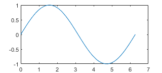 |
| 'tight' | Fit the axes box tightly around the data by setting the axis limits equal to the range of the data. | 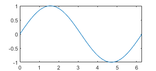 |
| 'padded' | Fit the axes box around the data with a thin margin of padding on each side. The width of the margin is approximately 7% of your data range. | 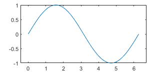 |
Note
The axis limit method has no effect when the corresponding mode property (XLimMode, YLimMode, or ZLimMode) is set to 'manual'.
XAxis, YAxis, ZAxis — Axis ruler
ruler object
Axis ruler, returned as a ruler object. The ruler controls the appearance and behavior of the _x_-axis,_y_-axis, or _z_-axis. Modify the appearance and behavior of a particular axis by accessing the associated ruler and setting ruler properties. The type of ruler that MATLAB creates for each axis depends on the plotted data. For a list of ruler properties, see:
- NumericRuler Properties
- DatetimeRuler Properties
- DurationRuler Properties
- CategoricalRuler Properties
For example, access the ruler for the _x_-axis through the XAxis property. Then, change theColor property of the ruler, and thus the color of the _x_-axis, to red. Similarly, change the color of the_y_-axis to green.
ax = gca; ax.XAxis.Color = 'r'; ax.YAxis.Color = 'g';
If the Axes object has two _y_-axes, then theYAxis property stores two ruler objects.
XAxisLocation — _x_-axis location
'bottom' (default) | 'top' | 'origin'
_x_-axis location, specified as one of the values in this table. This property applies only to 2-D views.
| Value | Description | Result |
|---|---|---|
| 'bottom' | Bottom of the axes.Example: ax.XAxisLocation = 'bottom' |  |
| 'top' | Top of the axes.Example: ax.XAxisLocation = 'top' |  |
| 'origin' | Through the origin point (0,0).Example: ax.XAxisLocation = 'origin' | 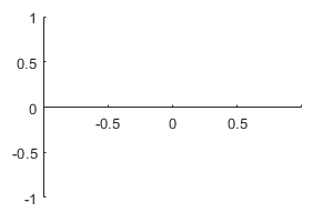 |
YAxisLocation — _y_-axis location
'left' (default) | 'right' | 'origin'
_y_-axis location, specified as one of the values in this table. This property applies only to 2-D views.
| Value | Description | Result |
|---|---|---|
| 'left' | Left side of the axes.Example: ax.YAxisLocation = 'left' | 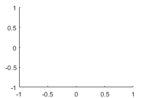 |
| 'right' | Right side of the axes.Example: ax.YAxisLocation = 'right' | 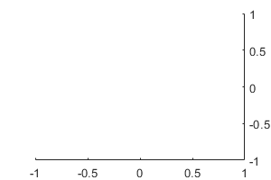 |
| 'origin' | Through the origin point (0,0).Example: ax.YAxisLocation = 'origin' | 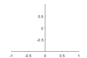 |
XColor, YColor, ZColor — Color of axis line, tick values, and labels
[0.15 0.15 0.15] (default) | RGB triplet | hexadecimal color code | 'r' | 'g' | 'b' | ...
Color of the axis line, tick values, and labels in the_x_, y, or_z_ direction, specified as an RGB triplet, a hexadecimal color code, a color name, or a short name. The color also affects the grid lines, unless you specify the grid line color using theGridColor or MinorGridColor property.
For a custom color, specify an RGB triplet or a hexadecimal color code.
- An RGB triplet is a three-element row vector whose elements specify the intensities of the red, green, and blue components of the color. The intensities must be in the range
[0,1], for example,[0.4 0.6 0.7]. - A hexadecimal color code is a string scalar or character vector that starts with a hash symbol (
#) followed by three or six hexadecimal digits, which can range from0toF. The values are not case sensitive. Therefore, the color codes"#FF8800","#ff8800","#F80", and"#f80"are equivalent.
Alternatively, you can specify some common colors by name. This table lists the named color options, the equivalent RGB triplets, and hexadecimal color codes.
| Color Name | Short Name | RGB Triplet | Hexadecimal Color Code | Appearance |
|---|---|---|---|---|
| "red" | "r" | [1 0 0] | "#FF0000" |  |
| "green" | "g" | [0 1 0] | "#00FF00" |  |
| "blue" | "b" | [0 0 1] | "#0000FF" |  |
| "cyan" | "c" | [0 1 1] | "#00FFFF" |  |
| "magenta" | "m" | [1 0 1] | "#FF00FF" |  |
| "yellow" | "y" | [1 1 0] | "#FFFF00" |  |
| "black" | "k" | [0 0 0] | "#000000" |  |
| "white" | "w" | [1 1 1] | "#FFFFFF" |  |
| "none" | Not applicable | Not applicable | Not applicable | No color |
Here are the RGB triplets and hexadecimal color codes for the default colors MATLAB uses in many types of plots.
| RGB Triplet | Hexadecimal Color Code | Appearance |
|---|---|---|
| [0 0.4470 0.7410] | "#0072BD" | ![Sample of RGB triplet [0 0.4470 0.7410], which appears as dark blue](https://www.mathworks.com/help/matlab/ref/colororder1.png) |
| [0.8500 0.3250 0.0980] | "#D95319" | ![Sample of RGB triplet [0.8500 0.3250 0.0980], which appears as dark orange](https://www.mathworks.com/help/matlab/ref/colororder2.png) |
| [0.9290 0.6940 0.1250] | "#EDB120" | ![Sample of RGB triplet [0.9290 0.6940 0.1250], which appears as dark yellow](https://www.mathworks.com/help/matlab/ref/colororder3.png) |
| [0.4940 0.1840 0.5560] | "#7E2F8E" | ![Sample of RGB triplet [0.4940 0.1840 0.5560], which appears as dark purple](https://www.mathworks.com/help/matlab/ref/colororder4.png) |
| [0.4660 0.6740 0.1880] | "#77AC30" | ![Sample of RGB triplet [0.4660 0.6740 0.1880], which appears as medium green](https://www.mathworks.com/help/matlab/ref/colororder5.png) |
| [0.3010 0.7450 0.9330] | "#4DBEEE" | ![Sample of RGB triplet [0.3010 0.7450 0.9330], which appears as light blue](https://www.mathworks.com/help/matlab/ref/colororder6.png) |
| [0.6350 0.0780 0.1840] | "#A2142F" | ![Sample of RGB triplet [0.6350 0.0780 0.1840], which appears as dark red](https://www.mathworks.com/help/matlab/ref/colororder7.png) |
Example: ax.XColor = [1 1 0]
Example: ax.YColor = 'yellow'
Example: ax.ZColor = '#FFFF00'
XColorMode — Property for setting _x_-axis grid color
'auto' (default) | 'manual'
Property for setting the _x_-axis grid color, specified as 'auto' or 'manual'. The mode value only affects the _x_-axis grid color. The_x_-axis line, tick values, and labels always use theXColor value, regardless of the mode.
The _x_-axis grid color depends on both theXColorMode property and theGridColorMode property, as shown here.
| XColorMode | GridColorMode | x-Axis Grid Color |
|---|---|---|
| 'auto' | 'auto' | GridColor property |
| 'manual' | GridColor property | |
| 'manual' | 'auto' | XColor property |
| 'manual' | GridColor property |
The _x_-axis minor grid color depends on both theXColorMode property and theMinorGridColorMode property, as shown here.
| XColorMode | MinorGridColorMode | x-Axis Minor Grid Color |
|---|---|---|
| 'auto' | 'auto' | MinorGridColor property |
| 'manual' | MinorGridColor property | |
| 'manual' | 'auto' | XColor property |
| 'manual' | MinorGridColor property |
YColorMode — Property for setting _y_-axis grid color
'auto' (default) | 'manual'
Property for setting the _y_-axis grid color, specified as 'auto' or 'manual'. The mode value only affects the _y_-axis grid color. The_y_-axis line, tick values, and labels always use theYColor value, regardless of the mode.
The _y_-axis grid color depends on both theYColorMode property and theGridColorMode property, as shown here.
| YColorMode | GridColorMode | y-Axis Grid Color |
|---|---|---|
| 'auto' | 'auto' | GridColor property |
| 'manual' | GridColor property | |
| 'manual' | 'auto' | YColor property |
| 'manual' | GridColor property |
The _y_-axis minor grid color depends on both theYColorMode property and theMinorGridColorMode property, as shown here.
| YColorMode | MinorGridColorMode | y-Axis Minor Grid Color |
|---|---|---|
| 'auto' | 'auto' | MinorGridColor property |
| 'manual' | MinorGridColor property | |
| 'manual' | 'auto' | YColor property |
| 'manual' | MinorGridColor property |
ZColorMode — Property for setting _z_-axis grid color
'auto' (default) | 'manual'
Property for setting the _z_-axis grid color, specified as 'auto' or 'manual'. The mode value only affects the _z_-axis grid color. The_z_-axis line, tick values, and labels always use theZColor value, regardless of the mode.
The _z_-axis grid color depends on both theZColorMode property and theGridColorMode property, as shown here.
| ZColorMode | GridColorMode | z-Axis Grid Color |
|---|---|---|
| 'auto' | 'auto' | GridColor property |
| 'manual' | GridColor property | |
| 'manual' | 'auto' | ZColor property |
| 'manual' | GridColor property |
The _z_-axis minor grid color depends on both theZColorMode property and theMinorGridColorMode property, as shown here.
| ZColorMode | MinorGridColorMode | z-Axis Minor Grid Color |
|---|---|---|
| 'auto' | 'auto' | MinorGridColor property |
| 'manual' | MinorGridColor property | |
| 'manual' | 'auto' | ZColor property |
| 'manual' | MinorGridColor property |
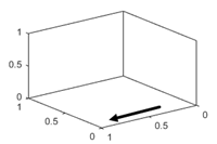
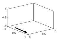
XDir — _x_-axis direction
'normal' (default) | 'reverse'
_x_-axis direction, specified as one of these values.
| Value | Description | Result in 2-D | Result in 3-D |
|---|---|---|---|
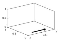
| 'normal' | Values increase from left to right.Example: ax.XDir = 'normal' | 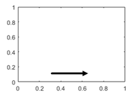 |
 |
| 'reverse' | Values increase from right to left.Example: ax.XDir = 'reverse' | 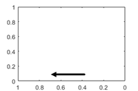 |
 |
YDir — _y_-axis direction
'normal' (default) | 'reverse'
_y_-axis direction, specified as one of these values.
| Value | Description | Result in 2-D | Result in 3-D |
|---|---|---|---|
| 'normal' | Values increase from bottom to top (2-D view) or front to back (3-D view).Example: ax.YDir = 'normal' | 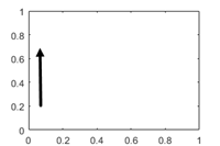 |
 |
| 'reverse' | Values increase from top to bottom (2-D view) or back to front (3-D view).Example: ax.YDir = 'reverse' | 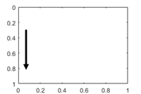 |
 |
ZDir — _z_-axis direction
'normal' (default) | 'reverse'
_z_-axis direction, specified as one of these values.
| Value | Description | Result in 3-D |
|---|---|---|
| 'normal' | Values increase pointing out of the screen (2-D view) or from bottom to top (3-D view).Example: ax.ZDir = 'normal' | 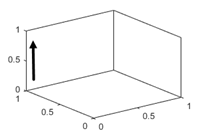 |
| 'reverse' | Values increase pointing into the screen (2-D view) or from top to bottom (3-D view).Example: ax.ZDir = 'reverse' | 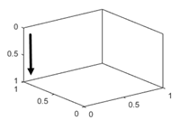 |
Axis scale, specified as one of these values.
| Value | Description | Result |
|---|---|---|
| 'linear' | Linear scaleExample: ax.XScale = 'linear' | 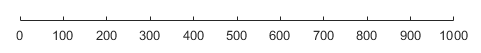 |
| 'log' | Log scaleExample: ax.XScale = 'log' NoteThe axes might exclude coordinates in some cases: If the coordinates include positive and negative values, only the positive values are displayed.If the coordinates are all negative, all of the values are displayed on a log scale with the appropriate sign.Zero values are not displayed. | 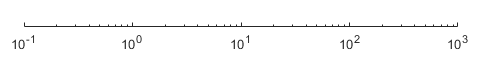 |
Grids
XGrid, YGrid, ZGrid — Grid lines
'off' (default) | on/off logical value
Grid lines, specified as 'on' or'off', or as numeric or logical 1 (true) or 0 (false). A value of 'on' is equivalent to true, and 'off' is equivalent to false. Thus, you can use the value of this property as a logical value. The value is stored as an on/off logical value of type matlab.lang.OnOffSwitchState.
'on'— Display grid lines perpendicular to the axis; for example, along lines of constant_x_, y, or_z_ values.'off'— Do not display the grid lines.
Alternatively, use the grid on or grid off command to set all three properties to'on' or 'off', respectively. For more information, see grid.
Example: ax.XGrid = 'on'
Placement of grid lines and tick marks in relation to graphic objects, specified as one of these values:
'bottom'— Display tick marks and grid lines under graphics objects.'top'— Display tick marks and grid lines over graphics objects.
This property affects only 2-D views.
Example: ax.Layer = 'top'
Line style for grid lines, specified as one of the line styles in this table.
| Line Style | Description | Resulting Line |
|---|---|---|
| "-" | Solid line |  |
| "--" | Dashed line |  |
| ":" | Dotted line |  |
| "-." | Dash-dotted line |  |
| "none" | No line | No line |
To display the grid lines, use the grid on command or set the XGrid, YGrid, orZGrid property to 'on'.
Example: ax.GridLineStyle = '--'
GridLineWidth — Grid line width
0.5 (default) | positive number
Since R2023a
Grid line width, specified as a positive number. Set this property or the MinorGridLineWidth property to control the thickness of the grid lines independently of the box outline and tick marks.
Example
Create vectors x and y, and plot them. Display the grid lines in the axes by calling grid on. Increase the thickness of the grid lines, box outline, and tick marks by setting theLineWidth property of the axes to1.5.
x = linspace(0,10); y = sin(x); plot(x,y) grid on ax = gca; ax.LineWidth = 1.5;
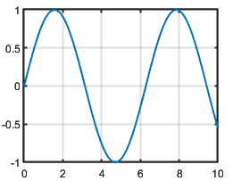
Make the grid lines thinner by setting the grid line width to 0.5.
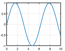
GridLineWidthMode — How grid line width is set
"auto" (default) | "manual"
Since R2023a
How the grid line width is set, specified as one of these values:
"auto"— Set theGridLineWidthproperty to the same value as theLineWidthproperty."manual"— Hold the current value of theGridLineWidthproperty.
MATLAB sets this property to "manual" when you explicitly set the GridLineWidth property to a value.
GridColor — Color of grid lines
[0.15 0.15 0.15] (default) | RGB triplet | hexadecimal color code | 'r' | 'g' | 'b' | ...
Color of grid lines, specified as an RGB triplet, a hexadecimal color code, a color name, or a short name.
For a custom color, specify an RGB triplet or a hexadecimal color code.
- An RGB triplet is a three-element row vector whose elements specify the intensities of the red, green, and blue components of the color. The intensities must be in the range
[0,1], for example,[0.4 0.6 0.7]. - A hexadecimal color code is a string scalar or character vector that starts with a hash symbol (
#) followed by three or six hexadecimal digits, which can range from0toF. The values are not case sensitive. Therefore, the color codes"#FF8800","#ff8800","#F80", and"#f80"are equivalent.
Alternatively, you can specify some common colors by name. This table lists the named color options, the equivalent RGB triplets, and hexadecimal color codes.
| Color Name | Short Name | RGB Triplet | Hexadecimal Color Code | Appearance |
|---|---|---|---|---|
| "red" | "r" | [1 0 0] | "#FF0000" | |
| "green" | "g" | [0 1 0] | "#00FF00" | |
| "blue" | "b" | [0 0 1] | "#0000FF" | |
| "cyan" | "c" | [0 1 1] | "#00FFFF" | |
| "magenta" | "m" | [1 0 1] | "#FF00FF" | |
| "yellow" | "y" | [1 1 0] | "#FFFF00" | |
| "black" | "k" | [0 0 0] | "#000000" | |
| "white" | "w" | [1 1 1] | "#FFFFFF" | |
| "none" | Not applicable | Not applicable | Not applicable | No color |
Here are the RGB triplets and hexadecimal color codes for the default colors MATLAB uses in many types of plots.
| RGB Triplet | Hexadecimal Color Code | Appearance |
|---|---|---|
| [0 0.4470 0.7410] | "#0072BD" | |
| [0.8500 0.3250 0.0980] | "#D95319" | |
| [0.9290 0.6940 0.1250] | "#EDB120" | |
| [0.4940 0.1840 0.5560] | "#7E2F8E" | |
| [0.4660 0.6740 0.1880] | "#77AC30" | |
| [0.3010 0.7450 0.9330] | "#4DBEEE" | |
| [0.6350 0.0780 0.1840] | "#A2142F" | |
To set the colors for the axes box outline, use theXColor, YColor, andZColor properties.
To display the grid lines, use the grid on command or set the XGrid, YGrid, orZGrid property to 'on'.
Example: ax.GridColor = [0 0 1]
Example: ax.GridColor = 'blue'
Example: ax.GridColor = '#0000FF'
GridColorMode — Property for setting grid color
'auto' (default) | 'manual'
Property for setting the grid color, specified as one of these values:
'auto'— Check the values of theXColorMode,YColorMode, andZColorModeproperties to determine the grid line colors for the x,y, and z directions.'manual'— UseGridColorto set the grid line color for all directions.
Grid-line transparency, specified as a value in the range [0,1]. A value of 1 means opaque and a value of 0 means completely transparent.
Example: ax.GridAlpha = 0.5
Selection mode for the GridAlpha property, specified as one of these values:
'auto'— Default transparency value of0.15.'manual'— Manually specify the transparency value. To specify the value, set theGridAlphaproperty.
Example: ax.GridAlphaMode = 'auto'
XMinorGrid, YMinorGrid, ZMinorGrid — Minor grid lines
'off' (default) | on/off logical value
Minor grid lines, specified as 'on' or'off', or as numeric or logical 1 (true) or 0 (false). A value of 'on' is equivalent to true, and 'off' is equivalent to false. Thus, you can use the value of this property as a logical value. The value is stored as an on/off logical value of type matlab.lang.OnOffSwitchState.
'on'— Display grid lines aligned with the minor tick marks of the axis. You do not need to enable minor ticks to display minor grid lines.'off'— Do not display grid lines.
Alternatively, use the grid minor command to toggle the visibility of the minor grid lines.
Example: ax.XMinorGrid = 'on'
MinorGridLineStyle — Line style for minor grid lines
':' (default) | '-' | '--' | '-.' | 'none'
Line style for minor grid lines, specified as one of the line styles shown in this table.
| Line Style | Description | Resulting Line |
|---|---|---|
| "-" | Solid line | |
| "--" | Dashed line | |
| ":" | Dotted line | |
| "-." | Dash-dotted line | |
| "none" | No line | No line |
To display minor grid lines, use the grid minor command or set the XMinorGrid, YMinorGrid, or ZMinorGrid property to'on'.
Example: ax.MinorGridLineStyle = '-.'
MinorGridLineWidth — Minor grid line width
0.5 (default) | positive number
Since R2023a
Minor grid line width, specified as a positive number. Set this property or the GridLineWidth property to control the thickness of the grid lines independently of the box outline and tick marks.
Tip
- To see the minor grid lines, set the
XMinorGrid,YMinorGrid, orZMinorGridproperties to"on". - When you set the
GridLineWidthproperty, MATLAB also sets theMinorGridLineWidthproperty to the same value. To avoid changing theMinorGridLineWidthproperty, set theMinorGridLineWidthModeproperty to"manual"before setting theGridLineWidthproperty.
MinorGridLineWidthMode — How minor grid line width is set
"auto" (default) | "manual"
Since R2023a
How the minor grid line width is set, specified as one of these values:
"auto"— Set theMinorGridLineWidthproperty to the same value as theGridLineWidthproperty."manual"— Hold the current value of theMinorGridLineWidthproperty.
MATLAB sets this property to "manual" when you explicitly set the MinorGridLineWidth property to a value.
MinorGridColor — Color of minor grid lines
[0.1 0.1 0.1] (default) | RGB triplet | hexadecimal color code | 'r' | 'g' | 'b' | ...
Color of minor grid lines, specified as an RGB triplet, a hexadecimal color code, a color name, or a short name.
For a custom color, specify an RGB triplet or a hexadecimal color code.
- An RGB triplet is a three-element row vector whose elements specify the intensities of the red, green, and blue components of the color. The intensities must be in the range
[0,1], for example,[0.4 0.6 0.7]. - A hexadecimal color code is a string scalar or character vector that starts with a hash symbol (
#) followed by three or six hexadecimal digits, which can range from0toF. The values are not case sensitive. Therefore, the color codes"#FF8800","#ff8800","#F80", and"#f80"are equivalent.
Alternatively, you can specify some common colors by name. This table lists the named color options, the equivalent RGB triplets, and hexadecimal color codes.
| Color Name | Short Name | RGB Triplet | Hexadecimal Color Code | Appearance |
|---|---|---|---|---|
| "red" | "r" | [1 0 0] | "#FF0000" | |
| "green" | "g" | [0 1 0] | "#00FF00" | |
| "blue" | "b" | [0 0 1] | "#0000FF" | |
| "cyan" | "c" | [0 1 1] | "#00FFFF" | |
| "magenta" | "m" | [1 0 1] | "#FF00FF" | |
| "yellow" | "y" | [1 1 0] | "#FFFF00" | |
| "black" | "k" | [0 0 0] | "#000000" | |
| "white" | "w" | [1 1 1] | "#FFFFFF" | |
| "none" | Not applicable | Not applicable | Not applicable | No color |
Here are the RGB triplets and hexadecimal color codes for the default colors MATLAB uses in many types of plots.
| RGB Triplet | Hexadecimal Color Code | Appearance |
|---|---|---|
| [0 0.4470 0.7410] | "#0072BD" | |
| [0.8500 0.3250 0.0980] | "#D95319" | |
| [0.9290 0.6940 0.1250] | "#EDB120" | |
| [0.4940 0.1840 0.5560] | "#7E2F8E" | |
| [0.4660 0.6740 0.1880] | "#77AC30" | |
| [0.3010 0.7450 0.9330] | "#4DBEEE" | |
| [0.6350 0.0780 0.1840] | "#A2142F" | |
To display minor grid lines, use the grid minor command or set the XMinorGrid, YMinorGrid, or ZMinorGrid property to'on'.
Example: ax.MinorGridColor = [0 0 1]
Example: ax.MinorGridColor = 'blue'
Example: ax.MinorGridColor = '#0000FF'
MinorGridColorMode — Property for setting minor grid color
'auto' (default) | 'manual'
Property for setting the minor grid color, specified as one of these values:
'auto'— Check the values of theXColorMode,YColorMode, andZColorModeproperties to determine the grid line colors for the x,y, and z directions.'manual'— UseMinorGridColorto set the minor grid line color for all directions.
Minor grid line transparency, specified as a value in the range [0,1]. A value of 1 means opaque and a value of 0 means completely transparent.
Example: ax.MinorGridAlpha = 0.5
Selection mode for the MinorGridAlpha property, specified as one of these values:
'auto'— Default transparency value of0.25.'manual'— Manually specify the transparency value. To specify the value, set theMinorGridAlphaproperty.
Example: ax.MinorGridAlphaMode = 'auto'
Labels
Title — Text object for axes title
text object
Text object for axes title. To add a title, set theString property of the text object. To change the title appearance, such as the font style or color, set other properties. For a complete list, see Text Properties.
ax = uiaxes; ax.Title.String = 'My Graph Title'; ax.Title.FontWeight = 'normal';
Alternatively, use the title function to add a title and control the appearance.
title(ax,'My Title','FontWeight','normal')
Subtitle — Text object for subtitle
text object
Text object for the axes subtitle. To add a subtitle, set theString property of the text object. To change its appearance, such as the font angle, set other properties. For a complete list, see Text Properties.
ax = uiaxes; ax.Subtitle.String = 'An Insightful Subtitle'; ax.Subtitle.FontAngle = 'italic';
Alternatively, use either the subtitle function or the title function to add a subtitle and control the appearance.
% subtitle function subtitle(ax,'Insightful Subtitle','FontAngle','italic')
% title function [t,s] = title(ax,'Clever Title','Insightful Subtitle'); s.FontAngle = 'italic';
Note
This text object is not contained in the Children property of the UIAxes object. It cannot be returned by findobj, and it does not use the default values defined for text objects.
TitleHorizontalAlignment — Title and subtitle horizontal alignment
'center' (default) | 'left' | 'right'
Title and subtitle horizontal alignment with the plot box, specified as one of the values from the table.
| TitleHorizontalAlignment Value | Description | Appearance |
|---|---|---|
| 'center' | The title and subtitle are centered over the plot box. |  |
| 'left' | The title and subtitle are aligned with the left side of the plot box. | 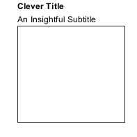 |
| 'right' | The title and subtitle are aligned with the right side of the plot box. | 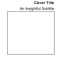 |
XLabel, YLabel, ZLabel — Text object for axis label
text object
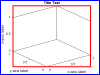
Text object for axis label. To add an axis label, set theString property of the text object. To change the label appearance, such as the font size, set other properties. For a complete list, see Text Properties.
ax = uiaxes; ax.YLabel.String = 'y-Axis Label'; ax.YLabel.FontSize = 12;
Alternatively, use the xlabel, ylabel, and zlabel functions to add an axis label and control the appearance.
ylabel(ax,'My y-Axis Label','FontSize',12)
Legend — Legend associated with axes
empty GraphicsPlaceholder (default) | Legend object
This property is read-only.
Legend associated with the UIAxes object, specified as aLegend object. To add a legend to the axes, use thelegend function. Then, you can use this property to modify the legend. For a complete list of properties, see Legend Properties.
ax = uiaxes; ax.Legend.TextColor = 'red';
You also can use this property to determine if the axes has a legend.
ax = uiaxes; lgd = ax.Legend if ~isempty(lgd) disp('Legend Exists') end
Multiple Plots
Color order, specified as a three-column matrix of RGB triplets. This property defines the palette of colors MATLAB uses to create plot objects such as Line,Scatter, and Bar objects. Each row of the array is an RGB triplet. An RGB triplet is a three-element vector whose elements specify the intensities of the red, green, and blue components of a color. The intensities must be in the range [0, 1]. This table lists the default colors.
This table lists the default colors.
| RGB Triplet | Hexadecimal Color Code | Appearance |
|---|---|---|
| [0 0.4470 0.7410] | "#0072BD" | |
| [0.8500 0.3250 0.0980] | "#D95319" | |
| [0.9290 0.6940 0.1250] | "#EDB120" | |
| [0.4940 0.1840 0.5560] | "#7E2F8E" | |
| [0.4660 0.6740 0.1880] | "#77AC30" | |
| [0.3010 0.7450 0.9330] | "#4DBEEE" | |
| [0.6350 0.0780 0.1840] | "#A2142F" | |
MATLAB assigns colors to objects according to their order of creation. For example, when plotting lines, the first line uses the first color, the second line uses the second color, and so on. If there are more lines than colors, then the cycle repeats.
Changing the Color Order Before or After Plotting
You can change the color order in either of the following ways:
- Call the colororder function to change the color order for all the axes in a figure. The colors of existing plots in the figure update immediately. If you place additional axes into the figure, those axes also use the new color order. If you continue to call plotting commands, those commands also use the new colors.
- Set the
ColorOrderproperty on the axes, call thehold function to set the axes hold state to'on', and then call the desired plotting functions. This is like calling thecolororderfunction, but in this case you are setting the color order for the specific axes, not the entire figure. Setting theholdstate to'on'is necessary to ensure that subsequent plotting commands do not reset the axes to use the default color order.
Color order index, specified as a positive integer. This property specifies the next color MATLAB selects from the axes ColorOrder property when it creates the next plot object such as a Line,Scatter, or Bar object.
Line style order, specified as a character vector, a cell array of character vectors, or a string array. This property lists the line styles that MATLAB uses to display multiple plot lines in the axes. MATLAB assigns styles to lines according to their order of creation. By default, it changes to the next line style only after cycling through all the colors in theColorOrder property with the current line style. Set the LineStyleCyclingMethod property to "withcolor" to cycle through both together or to"beforecolor" to cycle through the line styles first. The defaultLineStyleOrder has only one line style,"-".
To customize the line style order, create a cell array of character vectors or a string array. Specify each element of the array as a line specifier or marker specifier from the following tables. You can combine a line and a marker specifier into a single element, such as "-*".
| Line Style | Description | Resulting Line |
|---|---|---|
| "-" | Solid line | |
| "--" | Dashed line | |
| ":" | Dotted line | |
| "-." | Dash-dotted line | |
| Marker | Description | Resulting Marker |
|---|---|---|
| "o" | Circle |  |
| "+" | Plus sign |  |
| "*" | Asterisk |  |
| "." | Point |  |
| "x" | Cross |  |
| "_" | Horizontal line |  |
| "|" | Vertical line |  |
| "square" | Square |  |
| "diamond" | Diamond |  |
| "^" | Upward-pointing triangle |  |
| "v" | Downward-pointing triangle |  |
| ">" | Right-pointing triangle |  |
| "<" | Left-pointing triangle |  |
| "pentagram" | Pentagram |  |
| "hexagram" | Hexagram |  |
Changing Line Style Order Before or After Plotting
You can change the line style order before or after plotting into the axes. When you set the LineStyleOrder property to a new value, MATLAB updates the styles of any lines that are in the axes. If you continue plotting into the axes, your plotting commands continue using the line styles from the updated list.
LineStyleCyclingMethod — How to cycle through line styles
"aftercolor" (default) | "beforecolor" | "withcolor"
Since R2023a
How to cycle through the line styles when there are multiple lines in the axes, specified as one of the values from this table.
The examples in this table were created using the default colors in theColorOrder property and three line styles (["-","-o","--"]) in the LineStyleOrder property.
| Value | Description | Example |
|---|---|---|
| "aftercolor" | Cycle through the line styles of the LineStyleOrder after the colors of the ColorOrder. | 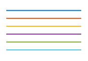 |
| "beforecolor" | Cycle through the line styles of theLineStyleOrder before the colors of theColorOrder. | 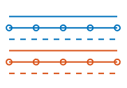 |
| "withcolor" | Cycle through the line styles of theLineStyleOrder with the colors of theColorOrder. | 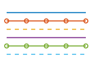 |
NextSeriesIndex — SeriesIndex value for next object
whole number
This property is read-only.
SeriesIndex value for the next plot object added to the axes, returned as a whole number greater than or equal to 0. This property is useful when you want to track how the objects cycle through the colors and line styles. This property maintains a count of the objects in the axes that have a numericSeriesIndex property value. MATLAB uses it to assign a SeriesIndex value to each new object. The count starts at 1 when you create the axes, and it increases by 1 for each additional object. Thus, the count is typically n+1, where n is the number of objects in the axes.
If you manually change the ColorOrderIndex orLineStyleOrderIndex property on the axes, the value of theNextSeriesIndex property changes to 0. As a consequence, objects that have a SeriesIndex property no longer update automatically when you change the ColorOrder orLineStyleOrder properties on the axes.
NextPlot — Properties to reset
'replacechildren' (default) | 'add' | 'replaceall' | 'replace'
Properties to reset when adding a new plot to the axes, specified as one of these values:
'add'— Add new plots to the existing axes. Do not delete existing plots or reset axes properties before displaying the new plot.'replacechildren'— Delete existing plots before displaying the new plot. Reset theColorOrderIndexandLineStyleOrderIndexproperties to1, but do not reset other axes properties. The next plot added to the axes uses the first color and line style based on theColorOrderandLineStyleorder properties. This value is similar to using cla before every new plot.'replace'— Delete existing plots and reset axes properties, exceptPositionandUnits, to their default values before displaying the new plot.'replaceall'— Delete existing plots and reset axes properties, exceptPositionandUnits, to their default values before displaying the new plot. This value is similar to usingcla resetbefore every new plot.
Note
- For
UIAxesobjects with only one_y_-axis, the'replace'and'replaceall'property values are equivalent. ForAxesobjects with two_y_-axes, the'replace'value affects only the active side while the'replaceall'value affects both sides. - Passing a
UIAxesobject to the cla function with the'reset'option sets theNextPlotproperty to'replace'unless you define a different default for theNextPlotproperty.
Figures created with the uifigure function also have a NextPlot property. Alternatively, you can use thenewplot function to prepare figures and axes for subsequent graphics commands.
Order for rendering objects, specified as one of these values:
'depth'— Draw objects in back-to-front order based on the current view. Use this value to ensure that objects in front of other objects are drawn correctly.'childorder'— Draw objects in the order in which they are created by graphics functions, without considering the relationship of the objects in three dimensions. This value can result in faster rendering, particularly if the figure is very large, but also can result in improper depth sorting of the objects displayed.
Line style order index, specified as a positive integer. This property specifies the next line style MATLAB selects from the axes LineStyleOrder property to create the next plot line.
Color and Transparency Maps
Colormap — Color map
parula (default) | m-by-3 array of RGB triplets
Color map, specified as an m-by-3 array of RGB (red, green, blue) triplets that define m individual colors.
Example: ax.Colormap = [1 0 1; 0 0 1; 1 1 0] sets the color map to three colors: magenta, blue, and yellow.
MATLAB accesses these colors by their row number.
Alternatively, use the colormap function to change the color map.
ColorScale — Scale for color mapping
'linear' (default) | 'log'
Scale for color mapping, specified as one of these values:
'linear'— Linear scale. The tick values along the colorbar also use a linear scale.'log'— Log scale. The tick values along the colorbar also use a log scale.
CLim — Color limits
[0 1] (default) | two-element vector of the form [cmin cmax]
Color limits for objects in axes that use the colormap, specified as a two-element vector of the form [cmin cmax]. This property determines how data values map to the colors in the colormap where:
cminspecifies the data value that maps to the first color in the colormap.cmaxspecifies the data value that maps to the last color in the colormap.
The Axes object interpolates data values between cmin and cmax across the colormap. Values outside this range use either the first or last color, whichever is closest.
Selection mode for the CLim property, specified as one of these values:
'auto'— Automatically select the limits based on the color data of the graphics objects contained in the axes.'manual'— Manually specify the values. To specify the values, set theCLimproperty. The values do not change when the limits of the axes children change.
Alphamap — Transparency map
array of 64 values from 0 to 1 (default) | array of finite alpha values from 0 to 1
Transparency map, specified as an array of finite alpha values that progress linearly from0 to 1. The size of the array can be_m_-by-1 or 1-by-m. MATLAB accesses alpha values by their index in the array. An alphamap can be any length.
AlphaScale — Scale for transparency mapping
'linear' (default) | 'log'
Scale for transparency mapping, specified as one of these values:
'linear'— Linear scale'log'— Log scale
ALim — Alpha limits
[0 1] (default) | two-element vector of the form [amin amax]
Alpha limits, specified as a two-element vector of the form [amin amax]. This property affects theAlphaData values of graphics objects, such as surface, image, and patch objects. This property determines how theAlphaData values map to the figure alpha map, where:
aminspecifies the data value that maps to the first alpha value in the figure alpha map.amaxspecifies the data value that maps to the last alpha value in the figure alpha map.
The UIAxes object interpolates data values betweenamin and amax across the figure alpha map. Values outside this range use either the first or last alpha map value, whichever is closest.
The Alphamap property of the figure contains the alpha map. For more information, see thealpha function.
Selection mode for the ALim property, specified as one of these values:
'auto'— Automatically select the limits based on theAlphaDatavalues of the graphics objects contained in the axes.'manual'— Manually specify the alpha limits. To specify the alpha limits, set theALimproperty.
Box Styling
Color — Color of plot area
[1 1 1] (default) | RGB triplet | hexadecimal color code | 'r' | 'g' | 'b' | ...
Color of plot area, specified as an RGB triplet, a hexadecimal color code, a color name, or a short name. The color affects the area defined by theInnerPosition property value.
For a custom color, specify an RGB triplet or a hexadecimal color code.
- An RGB triplet is a three-element row vector whose elements specify the intensities of the red, green, and blue components of the color. The intensities must be in the range
[0,1], for example,[0.4 0.6 0.7]. - A hexadecimal color code is a string scalar or character vector that starts with a hash symbol (
#) followed by three or six hexadecimal digits, which can range from0toF. The values are not case sensitive. Therefore, the color codes"#FF8800","#ff8800","#F80", and"#f80"are equivalent.
Alternatively, you can specify some common colors by name. This table lists the named color options, the equivalent RGB triplets, and hexadecimal color codes.
| Color Name | Short Name | RGB Triplet | Hexadecimal Color Code | Appearance |
|---|---|---|---|---|
| "red" | "r" | [1 0 0] | "#FF0000" | |
| "green" | "g" | [0 1 0] | "#00FF00" | |
| "blue" | "b" | [0 0 1] | "#0000FF" | |
| "cyan" | "c" | [0 1 1] | "#00FFFF" | |
| "magenta" | "m" | [1 0 1] | "#FF00FF" | |
| "yellow" | "y" | [1 1 0] | "#FFFF00" | |
| "black" | "k" | [0 0 0] | "#000000" | |
| "white" | "w" | [1 1 1] | "#FFFFFF" | |
| "none" | Not applicable | Not applicable | Not applicable | No color |
Here are the RGB triplets and hexadecimal color codes for the default colors MATLAB uses in many types of plots.
| RGB Triplet | Hexadecimal Color Code | Appearance |
|---|---|---|
| [0 0.4470 0.7410] | "#0072BD" | |
| [0.8500 0.3250 0.0980] | "#D95319" | |
| [0.9290 0.6940 0.1250] | "#EDB120" | |
| [0.4940 0.1840 0.5560] | "#7E2F8E" | |
| [0.4660 0.6740 0.1880] | "#77AC30" | |
| [0.3010 0.7450 0.9330] | "#4DBEEE" | |
| [0.6350 0.0780 0.1840] | "#A2142F" | |
Example: ax.Color = [0 0 1]
Example: ax.Color = 'blue'
Example: ax.Color = '#0000FF'
BackgroundColor — Color of margin around plot area
'none'
Color of margin around plot area, returned as 'none'.
Note
Setting this property has no effect.
LineWidth — Line width
0.5 (default) | positive numeric value
Line width of axes outline, tick marks, and grid lines, specified as a positive numeric value in point units. One point equals 1/72 inch.
Example: ax.LineWidth = 1.5
Box — Box outline
'off' (default) | on/off logical value
Box outline, specified as 'on' or'off', or as numeric or logical 1 (true) or 0 (false). A value of 'on' is equivalent to true, and 'off' is equivalent to false. Thus, you can use the value of this property as a logical value. The value is stored as an on/off logical value of type matlab.lang.OnOffSwitchState.
| Value | Description | 2-D Result | 3-D Result |
|---|---|---|---|
| 'on' | Display the box outline around the axes. For 3-D views, use the BoxStyle property to change extent of the outline.Example: ax.Box = 'on' |  |
 |
| 'off' | Do not display the box outline around the axes.Example: ax.Box = 'off' |  |
 |
The XColor,YColor, and ZColor properties control the color of the outline.
Example: ax.Box = 'on'
BoxStyle — Box outline style
'back' (default) | 'full'
Box outline style, specified as 'back' or'full'. This property affects only 3-D views.
| Value | Description | Result |
|---|---|---|
| 'back' | Outline the back planes of the 3-D box.Example: ax.BoxStyle = 'back' |  |
| 'full' | Outline the entire 3-D box.Example: ax.BoxStyle = 'full' |  |
Clipping — Clipping of objects to axes limits
'on' (default) | on/off logical value
Clipping of objects to the axes limits, specified as'on' or 'off', or as numeric or logical 1 (true) or0 (false). A value of'on' is equivalent to true, and'off' is equivalent to false. Thus, you can use the value of this property as a logical value. The value is stored as an on/off logical value of type matlab.lang.OnOffSwitchState.
The clipping behavior of an object within the Axes object depends on both the Clipping property of the Axes object and theClipping property of the individual object. The property value of the Axes object has these effects:
'on'— Enable each individual object within the axes to control its own clipping behavior based on theClippingproperty value for the object.'off'— Disable clipping for all objects within the axes, regardless of theClippingproperty value for the individual objects. Parts of objects can appear outside of the axes limits. For example, parts can appear outside the limits if you create a plot, use thehold oncommand, freeze the axis scaling, and then add a plot that is larger than the original plot.
This table lists the results for different combinations ofClipping property values.
| Clipping Property for Axes Object | Clipping Property for Individual Object | Result |
|---|---|---|
| 'on' | 'on' | Individual object is clipped. Others might or might not be. |
| 'on' | 'off' | Individual object is not clipped. Others might or might not be. |
| 'off' | 'on' | All objects are unclipped. |
| 'off' | 'off' | All objects are unclipped. |
ClippingStyle — Clipping boundaries
'3dbox' (default) | 'rectangle'
Clipping boundaries, specified as one of the values in this table. If a plot contains markers, then as long as the data point lies within the axes limits, MATLAB draws the entire marker.
The ClippingStyle property has no effect if theClipping property is set to'off'.
| Value | Descriptions | Illustration of Boundary Region |
|---|---|---|
| '3dbox' | Clip plotted objects to the six sides of the axes box defined by the axis limits.Thick lines might display outside the axes limits. |  |
| 'rectangle' | Clip plotted objects to a rectangular boundary enclosing the axes in any given view.Clip thick lines at the axes limits. |  |
AmbientLightColor — Background light color
[1 1 1] (default) | RGB triplet | hexadecimal color code | 'r' | 'g' | 'b' | ...
Background light color, specified as an RGB triplet, a hexadecimal color code, a color name, or a short name. The background light is a directionless light that shines uniformly on all objects in the axes. To add light, use the light function.
For a custom color, specify an RGB triplet or a hexadecimal color code.
- An RGB triplet is a three-element row vector whose elements specify the intensities of the red, green, and blue components of the color. The intensities must be in the range
[0,1], for example,[0.4 0.6 0.7]. - A hexadecimal color code is a string scalar or character vector that starts with a hash symbol (
#) followed by three or six hexadecimal digits, which can range from0toF. The values are not case sensitive. Therefore, the color codes"#FF8800","#ff8800","#F80", and"#f80"are equivalent.
Alternatively, you can specify some common colors by name. This table lists the named color options, the equivalent RGB triplets, and hexadecimal color codes.
| Color Name | Short Name | RGB Triplet | Hexadecimal Color Code | Appearance |
|---|---|---|---|---|
| "red" | "r" | [1 0 0] | "#FF0000" | |
| "green" | "g" | [0 1 0] | "#00FF00" | |
| "blue" | "b" | [0 0 1] | "#0000FF" | |
| "cyan" | "c" | [0 1 1] | "#00FFFF" | |
| "magenta" | "m" | [1 0 1] | "#FF00FF" | |
| "yellow" | "y" | [1 1 0] | "#FFFF00" | |
| "black" | "k" | [0 0 0] | "#000000" | |
| "white" | "w" | [1 1 1] | "#FFFFFF" | |
| "none" | Not applicable | Not applicable | Not applicable | No color |
Here are the RGB triplets and hexadecimal color codes for the default colors MATLAB uses in many types of plots.
| RGB Triplet | Hexadecimal Color Code | Appearance |
|---|---|---|
| [0 0.4470 0.7410] | "#0072BD" | |
| [0.8500 0.3250 0.0980] | "#D95319" | |
| [0.9290 0.6940 0.1250] | "#EDB120" | |
| [0.4940 0.1840 0.5560] | "#7E2F8E" | |
| [0.4660 0.6740 0.1880] | "#77AC30" | |
| [0.3010 0.7450 0.9330] | "#4DBEEE" | |
| [0.6350 0.0780 0.1840] | "#A2142F" | |
Example: ax.AmbientLightColor = [1 0 1]
Example: ax.AmbientLightColor = 'magenta'
Example: ax.AmbientLightColor = '#FF00FF'
Position
Size and location of axes, including the labels and margins, specified as a four-element vector of the form [left bottom width height]. This property is equivalent to the OuterPosition property. The vector defines a rectangle that encloses the outer bounds of the axes. The values are measured in the units specified by the Units property, which defaults to pixels.
- The
leftandbottomelements define the position of the rectangle, measured from the lower left corner of the parent container. - The
widthandheightdefine the size of the rectangle.
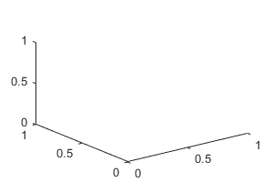
If you want to specify the position and account for the text around the axes, then set the either the Position or the OuterPosition property. These figures show the areas defined by the Position (orOuterPosition) in blue, and theInnerPosition in red.
| 2-D View of Axes | 3-D View of Axes |
|---|---|
 |
 |
Note
Setting this property has no effect when the parent container is aTiledChartLayout object.
InnerPosition — Size and location of inner axes, excluding labels and margins
[31.75 29.73 369.24 272.27] (default) | four-element vector
Inner size and location, excluding labels and margins, specified as a four-element vector of the form [left bottom width height]. The values are measured in the units specified by theUnits property, which defaults to pixels.
- The
leftandbottomelements define the position of the rectangle, measured from the lower left corner of the parent container. - The
widthandheightdefine the size of the rectangle.
If you want to specify the position and account for the text around the axes, then set the either the Position or theOuterPosition property. These figures show the areas defined by the Position (orOuterPosition) in blue, and theInnerPosition in red.
| 2-D View of Axes | 3-D View of Axes |
|---|---|
|
|
MATLAB automatically sets InnerPosition to the largest possible values that conform to all other properties. Other UIAxes properties that affect the axes size and shape include Position,DataAspectRatio andPlotBoxAspectRatio.
Note
- When querying the inner position of axes with constrained aspect ratios (such square axes or those containing images) consider using the tightPosition function for more accuracy.(since R2022b)
- Setting this property has no effect when the parent container is a
TiledChartLayout
OuterPosition — Size and location of axes, including labels and margins
[10 10 400 300] (default) | four-element vector
Size and location of the axes, including the labels and margins, specified as a four-element vector of the form [left bottom width height].
This property value is identical to the Position property value.
TightInset — Margin for text labels
four-element vector of the form [left bottom right top]
This property is read-only.
Margin for text labels, returned as a four-element vector of the form[left bottom right top]. The elements define the distances between the bounds of the InnerPosition property and the extent of the axes text labels and title. By default, the values are measured in pixels. To change the units, set theUnits property.
PositionConstraint — Position to hold constant
"outerposition" | "innerposition"
Position property to hold constant when adding, removing, or changing decorations, specified as one of the following values:
"outerposition"— TheOuterPositionproperty remains constant when you add, remove, or change decorations such as a title or an axis label. If any positional adjustments are needed, MATLAB adjusts theInnerPositionproperty."innerposition"— TheInnerPositionproperty remains constant when you add, remove, or change decorations such as a title or an axis label. If any positional adjustments are needed, MATLAB adjusts theOuterPositionproperty.
Note
Setting this property has no effect when the parent container is aTiledChartLayout object.
Units — Position units
'pixels' (default) | 'normalized' | 'inches' | 'centimeters' | 'points' | 'characters'
Position units, specified as one of these values.
| Units | Description |
|---|---|
| 'normalized' | Normalized with respect to the container, which is typically the figure or a panel. The lower left corner of the container maps to (0,0) and the upper right corner maps to(1,1). |
| 'inches' | Inches. |
| 'centimeters' | Centimeters. |
| 'characters' | Based on the default uicontrol font of the graphics root object: Character width = width of letterx.Character height = distance between the baselines of two lines of text. |
| 'points' | Typography points. One point equals 1/72 inch. |
| 'pixels' | On Windows systems, a pixel is 1/96th of an inch.On Macintosh systems, a pixel is 1/72nd of an inch.On Linux systems, the size of a pixel is determined by your system resolution. |
When specifying the units as a Name,Value pair during object creation, you must set the Units property before specifying the properties that you want to use these units, such asPosition.
DataAspectRatio — Relative length of data units
[1 1 1] (default) | three-element vector of the form [dx dy dz]
Relative length of data units along each axis, specified as a three-element vector of the form [dx dy dz]. This vector defines the relative x, y, and_z_ data scale factors. For example, specifying this property as [1 2 1] sets the length of one unit of data in the _x_-direction to be the same length as two units of data in the _y_-direction and one unit of data in the_z_-direction.
Alternatively, use the daspect function to change the data aspect ratio.
Example: ax.DataAspectRatio = [1 1 1]
Data Types: single | double | int8 | int16 | int32 | int64 | uint8 | uint16 | uint32 | uint64
DataAspectRatioMode — Data aspect ratio mode
'auto' (default) | 'manual'
Data aspect ratio mode, specified as one of these values:
'auto'— Automatically select values that make best use of the available space. IfPlotBoxAspectRatioModeandCameraViewAngleModeare also set to'auto', then enable "stretch-to-fill" behavior. Stretch the axes so that it fills the available space as defined by thePositionproperty.'manual'— Disable the "stretch-to-fill" behavior and use the manually specified data aspect ratio. To specify the values, set theDataAspectRatioproperty.
PlotBoxAspectRatio — Relative length of each axis
three-element vector of the form [px py pz]
Relative length of each axis, specified as a three-element vector of the form [px py pz] defining the relative_x_-axis, _y_-axis, and_z_-axis scale factors. The plot box is a box enclosing the axes data region as defined by the axis limits.
Alternatively, use the pbaspect function to change the data aspect ratio.
If you specify the axis limits, data aspect ratio, and plot box aspect ratio, then MATLAB ignores the plot box aspect ratio. It adheres to the axis limits and data aspect ratio.
Example: ax.PlotBoxAspectRatio = [1 0.75 0.75]
Data Types: single | double | int8 | int16 | int32 | int64 | uint8 | uint16 | uint32 | uint64
PlotBoxAspectRatioMode — Selection mode for PlotBoxAspectRatio
'auto' (default) | 'manual'
Selection mode for the PlotBoxAspectRatio property, specified as one of these values:
'auto'— Automatically select values that make best use of the available space. IfDataAspectRatioModeandCameraViewAngleModealso are set to'auto', then enable "stretch-to-fill" behavior. Stretch theAxesobject so that it fills the available space as defined by thePositionproperty.'manual'— Disable the "stretch-to-fill" behavior and use the manually specified plot box aspect ratio. To specify the values, set thePlotBoxAspectRatioproperty.
Layout — Layout options
empty LayoutOptions array (default) | GridLayoutOptions object | TiledChartLayoutOptions object
Layout options, specified as aGridLayoutOptions orTiledChartLayoutOptions object. This property specifies options when the axes is in a grid layout or a tiled chart layout. If the axes is not in either type of layout, then this property is empty and has no effect.
To position the axes in a specific row and column of a grid layout, set the Row and Column properties on the GridLayoutOptions object. For example, this code places the axes in the third row and second column of a grid layout.
g = uigridlayout([4 3]); ax = uiaxes(g); ax.Layout.Row = 3; ax.Layout.Column = 2;
To make the axes span multiple rows or columns, specify theRow or Column property as a two-element vector. For example, this axes spans columns2 through3:
ax.Layout.Column = [2 3];
View
View — Azimuth and elevation of view
[0 90] (default) | two-element vector of the form [azimuth elevation]
Azimuth and elevation of view, specified as a two-element vector of the form [azimuth elevation] defined in degree units. Alternatively, use the view function to set the view.
Note
Setting the azimuth and elevation angles might reset other camera-related properties. For best results, set the azimuth and elevation angles before setting other camera-related properties.
Example: ax.View = [45 45]
Projection — Type of projection onto 2-D screen
'orthographic' (default) | 'perspective'
Type of projection onto a 2-D screen, specified as one of these values:
'orthographic'— Maintain the correct relative dimensions of graphics objects regarding the distance of a given point from the viewer, and draw lines that are parallel in the data parallel on the screen.'perspective'— Incorporate foreshortening, which enables you to perceive depth in 2-D representations of 3-D objects. Perspective projection does not preserve the relative dimensions of objects. Instead, it displays a distant line segment smaller than a nearer line segment of the same length. Lines that are parallel in the data might not appear parallel on screen.
CameraPosition — Camera location
three-element vector of the form [x y z]
Camera location, or the viewpoint, specified as a three-element vector of the form [x y z]. This vector defines the axes coordinates of the camera location, which is the point from which you view the axes. The camera is oriented along the view axis, which is a straight line that connects the camera position and the camera target. For an illustration, see Camera Graphics Terminology.
If the Projection property is set to 'perspective', then as you change theCameraPosition setting, the amount of perspective also changes.
Alternatively, use the campos function to set the camera location.
Example: ax.CameraPosition = [0.5 0.5 9]
Data Types: single | double
CameraPositionMode — Selection mode for CameraPosition
'auto' (default) | 'manual'
Selection mode for the CameraPosition property, specified as one of these values:
'auto'— Automatically setCameraPositionalong the view axis. Calculate the position so that the camera lies a fixed distance from the target along the azimuth and elevation specified by the current view, as returned by the view function. Functions like rotate3d,zoom, and pan, change this mode to'auto'to perform their actions.'manual'— Manually specify the value. To specify the value, set theCameraPositionproperty.
CameraTarget — Camera target point
three-element vector of the form [x y z]
Camera target point, specified as a three-element vector of the form[x y z]. This vector defines the axes coordinates of the point. The camera is oriented along the view axis, which is a straight line that connects the camera position and the camera target. For an illustration, see Camera Graphics Terminology.
Alternatively, use the camtarget function to set the camera target.
Example: ax.CameraTarget = [0.5 0.5 0.5]
Data Types: single | double
CameraTargetMode — Selection mode for CameraTarget
'auto' (default) | 'manual'
Selection mode for the CameraTarget property, specified as one of these values:
'auto'— Position the camera target at the centroid of the axes plot box.'manual'— Use the manually specified camera target value. To specify a value, set theCameraTargetproperty.
CameraUpVector — Vector defining upwards direction
three-element direction vector of the form [x y z]
Vector defining upwards direction, specified as a three-element direction vector of the form [x y z]. For 2-D views, the default value is [0 1 0]. For 3-D views, the default value is[0 0 1]. For an illustration, see Camera Graphics Terminology.
Alternatively, use the camup function to set the upwards direction.
Example: ax.CameraUpVector = [sin(45) cos(45) 1]
CameraUpVectorMode — Selection mode for CameraUpVector
'auto' (default) | 'manual'
Selection mode for the CameraUpVector property, specified as one of these values:
'auto'— Automatically set the value to[0 0 1]for 3-D views so that the positive_z_-direction is up. Set the value to[0 1 0]for 2-D views so that the positive_y_-direction is up.'manual'— Manually specify the vector defining the upwards direction. To specify a value, set theCameraUpVector property.
CameraViewAngle — Field of view
6.6086 (default) | scalar angle in range [0,180)
Field of view, specified as a scalar angle greater than 0 and less than or equal to 180. Changing the camera view angle affects the size of graphics objects displayed in the axes, but does not affect the degree of perspective distortion. The greater the angle, the larger the field of view and the smaller objects appear in the scene. For an illustration, see Camera Graphics Terminology.
Example: ax.CameraViewAngle = 15
Data Types: single | double | int8 | int16 | int32 | int64 | uint8 | uint16 | uint32 | uint64 | logical
CameraViewAngleMode — Selection mode for CameraViewAngle
'auto' (default) | 'manual'
Selection mode for the CameraViewAngle property, specified as one of these values:
'auto'— Automatically select the field of view as the minimum angle that captures the entire scene, up to 180 degrees.'manual'— Manually specify the field of view. To specify a value, set the CameraViewAngle property.
Interactivity
InteractionOptions — Options to customize interaction behavior
CartesianAxesInteractionOptions object
Options to customize interaction behavior, specified as aCartesianAxesInteractionOptions object. Use the properties of the CartesianAxesInteractionOptions object to customize the behavior of interactions with the axes. For a complete list of properties, see CartesianAxesInteractionOptions Properties.
Before R2024a: Specify this property as anInteractionOptions object instead of as aCartesianAxesInteractionOptions object.
The options set by the CartesianAxesInteractionOptions object apply to these interactions on the associated axes:
- The built-in interactions specified by the Interactions property of the axes
- Interactions enabled by using mode functions, such aspan andzoom
- Interactions enabled using the axes toolbar
Example: ax.InteractionOptions.LimitsDimensions = "x" constrains all pan and zoom interactions to the_x_-dimension.
Toolbar — Toolbar with individual interaction buttons
AxesToolbar object (default) | []
Toolbar with individual interaction buttons, specified as anAxesToolbar object or an empty array. Use this property to customize the appearance and behavior of the toolbar. Create the toolbar using the axtoolbar function. The toolbar appears at the top-right corner of the UI axes when you hover over it.

The toolbar buttons depend on the contents of the UI axes, but typically include zooming, panning, rotating, brushing, exporting, and restoring the original view. You can customize the toolbar buttons using the axtoolbar and axtoolbarbtn functions.
For a complete list of properties, see AxesToolbar Properties.
To remove the toolbar, set this property to an empty array.
Interactions — Built-in interactions
array of interaction objects | []
Built-in interactions, specified as an array of interaction objects or an empty array. These interactions are available within your chart through gestures. You do not have to select any axes toolbar buttons to use them.
The default set of built-in interactions depends on the chart type. You can replace the default set with a new set of interactions, but you cannot access or modify the default set of interactions.
To remove all interactions from the axes, set this property to an empty array. To temporarily disable the current set of interactions, call thedisableDefaultInteractivity function. You can reenable them by calling the enableDefaultInteractivity function.
For a list of interaction objects, see Customize Built-In Interactions.
Example: ax.Interactions = [panInteraction zoomInteraction] replaces the default set of built-in interactions with the panInteraction and zoomInteraction objects. This set of interactions enables dragging to pan within the chart and scrolling to zoom within the chart.
Visible — State of visibility
'on' (default) | on/off logical value
State of visibility, specified as 'on' or 'off', or as numeric or logical 1 (true) or 0 (false). A value of 'on' is equivalent to true, and 'off' is equivalent to false. Thus, you can use the value of this property as a logical value. The value is stored as an on/off logical value of type matlab.lang.OnOffSwitchState.
'on'— Display the axes and its children.'off'— Hide the axes without deleting it. You still can access the properties of an invisible axes object.
Note
When the Visible property is 'off', the axes object is invisible, but child objects such as lines remain visible.
CurrentPoint — Location of mouse pointer
2-by-3 array
Location of mouse pointer, specified as a 2-by-3 array. TheCurrentPoint property contains the (x,y,z) coordinates of the mouse pointer with respect to the axes. The returned array is of the form:
[xfront yfront zfront xback yback zback]
The two points indicate the location of the last mouse click. However, if the figure has a WindowButtonMotionFcn callback defined, then the points indicate the last location of the mouse pointer. The figure also has a CurrentPoint property.
The values of the current point when using perspective projection can be different from the same point in orthographic projection because the shape of the axes volume can be different.
Orthogonal Projection
When using orthogonal projection, the values depend on whether the click is within the axes or outside the axes.
- If the click is inside the axes, the two points lie on the line that is perpendicular to the plane of the screen and that passes through the pointer. The coordinates are the points where this line intersects the front and back surfaces of the axes volume (which is defined by the axes x, y, and z limits). The first row is the point nearest to the camera position. The second row is the point farthest from the camera position. This is true for both 2-D and 3-D views.
- If the click is outside the axes, but within the figure, then the points lie on a line that passes through the pointer and is perpendicular to the camera target and camera position planes. The first row is the point in the camera position plane. The second row is the point in the plane of the camera target.
Perspective Projection
Clicking outside of the UIAxes object in perspective projection returns the front point as the current camera position. Only the back point updates with the coordinates of a point that lies on a line extending from the camera position through the pointer and intersecting the camera target at that point.
Context menu, specified as a ContextMenu object. Use this property to display a context menu when you right-click the object. Create the context menu using the uicontextmenu function.
Note
If the PickableParts property is set to'none' or if the HitTest property is set to 'off', then the context menu does not appear.
Selection state, specified as 'on' or 'off', or as numeric or logical 1 (true) or0 (false). A value of 'on' is equivalent to true, and 'off' is equivalent tofalse. Thus, you can use the value of this property as a logical value. The value is stored as an on/off logical value of type matlab.lang.OnOffSwitchState.
'on'— Selected. If you click the object when in plot edit mode, then MATLAB sets itsSelectedproperty to'on'. If theSelectionHighlightproperty also is set to'on', then MATLAB displays selection handles around the object.'off'— Not selected.
Display of selection handles when selected, specified as 'on' or'off', or as numeric or logical 1 (true) or 0 (false). A value of 'on' is equivalent to true, and 'off' is equivalent to false. Thus, you can use the value of this property as a logical value. The value is stored as an on/off logical value of type matlab.lang.OnOffSwitchState.
'on'— Display selection handles when theSelectedproperty is set to'on'.'off'— Never display selection handles, even when theSelectedproperty is set to'on'.
Callbacks
Mouse-click callback, specified as one of these values:
- Function handle
- Cell array containing a function handle and additional arguments
- Character vector that is a valid MATLAB command or function, which is evaluated in the base workspace (not recommended)
Use this property to execute code when you click the object. If you specify this property using a function handle, then MATLAB passes two arguments to the callback function when executing the callback:
- Clicked object — Access properties of the clicked object from within the callback function.
- Event data — Empty argument. Replace it with the tilde character (
~) in the function definition to indicate that this argument is not used.
For more information on how to use function handles to define callback functions, see Create Callbacks for Graphics Objects.
Note
If the PickableParts property is set to 'none' or if the HitTest property is set to 'off', then this callback does not execute.
Object creation function, specified as one of these values:
- Function handle.
- Cell array in which the first element is a function handle. Subsequent elements in the cell array are the arguments to pass to the callback function.
- Character vector containing a valid MATLAB expression (not recommended). MATLAB evaluates this expression in the base workspace.
For more information about specifying a callback as a function handle, cell array, or character vector, see Callbacks in App Designer.
This property specifies a callback function to execute when MATLAB creates the object. MATLAB initializes all property values before executing the CreateFcn callback. If you do not specify the CreateFcn property, then MATLAB executes a default creation function.
Setting the CreateFcn property on an existing component has no effect.
If you specify this property as a function handle or cell array, you can access the object that is being created using the first argument of the callback function. Otherwise, use the gcbo function to access the object.
Object deletion function, specified as one of these values:
- Function handle.
- Cell array in which the first element is a function handle. Subsequent elements in the cell array are the arguments to pass to the callback function.
- Character vector containing a valid MATLAB expression (not recommended). MATLAB evaluates this expression in the base workspace.
For more information about specifying a callback as a function handle, cell array, or character vector, see Callbacks in App Designer.
This property specifies a callback function to execute when MATLAB deletes the object. MATLAB executes the DeleteFcn callback before destroying the properties of the object. If you do not specify the DeleteFcn property, then MATLAB executes a default deletion function.
If you specify this property as a function handle or cell array, you can access the object that is being deleted using the first argument of the callback function. Otherwise, use the gcbo function to access the object.
Callback Execution Control
Callback interruption, specified as 'on' or 'off', or as numeric or logical 1 (true) or0 (false). A value of 'on' is equivalent to true, and 'off' is equivalent tofalse. Thus, you can use the value of this property as a logical value. The value is stored as an on/off logical value of type matlab.lang.OnOffSwitchState.
This property determines if a running callback can be interrupted. There are two callback states to consider:
- The running callback is the currently executing callback.
- The interrupting callback is a callback that tries to interrupt the running callback.
MATLAB determines callback interruption behavior whenever it executes a command that processes the callback queue. These commands include drawnow, figure, uifigure, getframe, waitfor, and pause.
If the running callback does not contain one of these commands, then no interruption occurs. MATLAB first finishes executing the running callback, and later executes the interrupting callback.
If the running callback does contain one of these commands, then theInterruptible property of the object that owns the running callback determines if the interruption occurs:
- If the value of
Interruptibleis'off', then no interruption occurs. Instead, theBusyActionproperty of the object that owns the interrupting callback determines if the interrupting callback is discarded or added to the callback queue. - If the value of
Interruptibleis'on', then the interruption occurs. The next time MATLAB processes the callback queue, it stops the execution of the running callback and executes the interrupting callback. After the interrupting callback completes, MATLAB then resumes executing the running callback.
Note
Callback interruption and execution behave differently in these situations:
- If the interrupting callback is a
DeleteFcn,CloseRequestFcn, orSizeChangedFcncallback, then the interruption occurs regardless of theInterruptibleproperty value. - If the running callback is currently executing the
waitforfunction, then the interruption occurs regardless of theInterruptibleproperty value. - If the interrupting callback is owned by a
Timerobject, then the callback executes according to schedule regardless of theInterruptibleproperty value.
Note
When an interruption occurs, MATLAB does not save the state of properties or the display. For example, the object returned by the gca or gcf command might change when another callback executes.
Callback queuing, specified as 'queue' or 'cancel'. The BusyAction property determines how MATLAB handles the execution of interrupting callbacks. There are two callback states to consider:
- The running callback is the currently executing callback.
- The interrupting callback is a callback that tries to interrupt the running callback.
The BusyAction property determines callback queuing behavior only when both of these conditions are met:
- The running callback contains a command that processes the callback queue, such as drawnow, figure, uifigure, getframe, waitfor, or pause.
- The value of the
Interruptibleproperty of the object that owns the running callback is'off'.
Under these conditions, the BusyAction property of the object that owns the interrupting callback determines how MATLAB handles the interrupting callback. These are possible values of theBusyAction property:
'queue'— Puts the interrupting callback in a queue to be processed after the running callback finishes execution.'cancel'— Does not execute the interrupting callback.
Ability to capture mouse clicks, specified as one of these values:
'visible'— Capture mouse clicks only when visible. TheVisibleproperty must be set to'on'. TheHitTestproperty determines if theUIAxesobject responds to the click or if an ancestor does.'all'— Capture mouse clicks regardless of visibility. TheVisibleproperty can be set to'on'or'off'. TheHitTestproperty determines if theUIAxesobject responds to the click or if an ancestor does.'none'— Cannot capture mouse clicks. Clicking theUIAxesobject passes the click to the object below it in the current view of the figure window, which is typically the axes or the figure. TheHitTestproperty has no effect.
If you want an object to be clickable when it is underneath other objects that you do not want to be clickable, then set the PickableParts property of the other objects to 'none' so that the click passes through them.
Response to captured mouse clicks, specified as 'on' or'off', or as numeric or logical 1 (true) or 0 (false). A value of 'on' is equivalent to true, and 'off' is equivalent to false. Thus, you can use the value of this property as a logical value. The value is stored as an on/off logical value of type matlab.lang.OnOffSwitchState.
'on'— Trigger theButtonDownFcncallback of theUIAxesobject. If you have defined theContextMenuproperty, then invoke the context menu.'off'— Trigger the callbacks for the nearest ancestor of theUIAxesobject that meets one of these conditions:HitTestproperty is set to'on'.PickablePartsproperty is set to a value that enables the ancestor to capture mouse clicks.
Note
The PickableParts property determines if the UIAxes object can capture mouse clicks. If it cannot, then the HitTest property has no effect.
This property is read-only.
Deletion status, returned as an on/off logical value of type matlab.lang.OnOffSwitchState.
MATLAB sets the BeingDeleted property to'on' when the DeleteFcn callback begins execution. The BeingDeleted property remains set to'on' until the component object no longer exists.
Check the value of the BeingDeleted property to verify that the object is not about to be deleted before querying or modifying it.
Parent/Child
Parent — Parent container
Figure object | Panel object | Tab object | GridLayout object | TiledChartLayout object
Parent container, specified as a Figure,Panel, Tab, GridLayout, or TiledChartLayout object. If no container is specified, MATLAB calls the uifigure function to create a new Figure object that serves as the parent container.
Children, returned as an array of graphics objects. Use this property to view a list of the children or to reorder the children by setting the property to a permutation of itself.
You cannot add or remove children using the Children property. To add a child to this list, set the Parent property of the child graphics object to the UIAxes object.
Visibility of the object handle in the Children property of the parent, specified as one of these values:
"on"— Object handle is always visible."off"— Object handle is invisible at all times. This option is useful for preventing unintended changes by another function. SetHandleVisibilityto"off"to temporarily hide the handle during the execution of that function."callback"— Object handle is visible from within callbacks or functions invoked by callbacks, but not from within functions invoked from the command line. This option blocks access to the object at the command line, but permits callback functions to access it.
If the object is not listed in the Children property of the parent, then functions that obtain object handles by searching the object hierarchy or querying handle properties cannot return it. Examples of such functions include theget, findobj, gca, gcf, gco, newplot, cla, clf, and close functions.
Hidden object handles are still valid. Set the root ShowHiddenHandles property to "on" to list all object handles regardless of theirHandleVisibility property setting.
Identifiers
Type — Type of graphics object
'axes'
This property is read-only.
Type of graphics object returned as 'axes'.
Object identifier, specified as a character vector or string scalar. You can specify a unique Tag value to serve as an identifier for an object. When you need access to the object elsewhere in your code, you can use the findobj function to search for the object based on the Tag value.
User data, specified as any MATLAB array. For example, you can specify a scalar, vector, matrix, cell array, character array, table, or structure. Use this property to store arbitrary data on an object.
If you are working in App Designer, create public or private properties in the app to share data instead of using the UserData property. For more information, see Share Data Within App Designer Apps.
Version History
Introduced in R2016a
R2024a: Specify InteractionOptions as aCartesianAxesInteractionOptions object
The InteractionOptions object is now calledCartesianAxesInteractionOptions. The behavior remains the same. The name of the InteractionOptions property has not changed. Starting in R2024a, set the InteractionOptions property using aCartesianAxesInteractionOptions object.
R2023a: Control cycling of line styles using the LineStyleCyclingMethod property
Use the LineStyleCyclingMethod property to control how different lines are distinguished from one another in the axes.
R2023a: Specify grid line thickness using the GridLineWidth and MinorGridLineWidth properties
Change the thickness of grid lines independently of the box outline and tick marks by setting the GridLineWidth andMinorGridLineWidth properties of the axes. Before R2023a, the LineWidth property of the axes was the only property for controlling the grid line width. However, that property controlled the grid lines, box outline, and tick marks together. Now you can control the thickness of the grid lines separately.
R2023a: Control behavior of axes interactions using the InteractionOptions property
Use the InteractionOptions property to control the behavior of axes interactions, such as pan, zoom, and rotate.
R2022a: XTickLabelRotationMode, YTickLabelRotationMode, andZTickLabelRotationMode properties added
Control the selection mode for tick label rotation by setting theXTickLabelRotationMode,YTickLabelRotationMode, orZTickLabelRotationMode property.
R2021b: Remove tick marks by setting the TickDir property to "none"
You can remove all the tick marks from the axes by setting theTickDir property to "none".
R2021a: Control axis limits with the XLimitMethod, YLimitMethod, and ZLimitMethod properties
Control the axis limits for your plots by setting theXLimitMethod, YLimitMethod, orZLimitMethod on the axes.
R2020b: BackgroundColor property has no effect
Setting the BackgroundColor property on aUIAxes object no longer has any effect. Starting in R2020b, the area around the plot box is transparent regardless of the value of theBackgroundColor property.
To produce the same effect as setting the background color in previous releases, create a panel with the desired BackgroundColor value, and then place the UIAxes in the panel.
R2020b: UIAxes appear behind all other objects
The stacking order (also called the Z-order) of objects in the figure has changed so that UIAxes objects and their contents appear behind all UI components in the figure. This behavior is consistent with the behavior of other types of axes.
For example, this code creates a figure, a button, and then aUIAxes object.
fig = uifigure; b = uibutton(fig); uax = uiaxes(fig);
In R2020a, executing the preceding code displays the UIAxes in front of the button, as shown in the figure on the left. The figure on the right shows the behavior in R2020b, where the UIAxes appears behind UI components regardless of the order of creation.
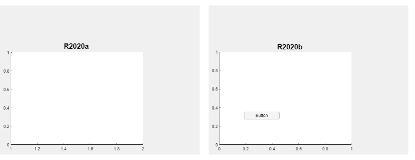
The order of the objects listed in the Children property of the figure also reflects this change. The UIAxes object is always after UI components in the list.
ans =
2×1 graphics array:
Button (Button) UIAxes
R2020b: Plots might extend outside the bounds of the axes
Plot objects such as lines might not clip to the bounds defined by theOuterPosition property of the UIAxes. The lines extend beyond the bounds when the Clipping property of each line is set to 'off'. In previous releases, the lines clip to the OuterPosition regardless of the value of theClipping property. For example, the plot on the left shows the R2020a behavior, and the plot on the right shows the R2020b behavior. In both cases, the Clipping properties of the lines are set to'off'.
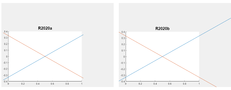
To prevent the axes content from overlapping with components in your app, set theClipping property of each object in the axes to'on'.
R2020b: UIAxes SizeChangedFcn callback has been removed
The SizeChangedFcn callback for UIAxes objects has been removed. If your app requires a callback that executes when the size of the axes changes, create a SizeChangedFCn callback for the parent figure or another container.
R2020b: Colorbars and legends displayed with UIAxes have the same parent as UIAxes
When you create a plot in a UIAxes object, and then create a colorbar or legend for that plot, the parent object of the colorbar or legend is the same as the parent object of the UIAxes object. In previous releases, the parent object of the colorbar or legend is theUIAxes object.
R2020b: Control the alignment of a plot title with the TitleHorizontalAlignment property
You can control the alignment of a plot title by setting theTitleHorizontalAlignment property of the axes to"left", "right", or"center".
R2020b: Create and style subtitles with the Subtitle and SubtitleFontWeight properties
Add a subtitle to your plot by setting the Subtitle property or calling the subtitle function. To control the appearance of the subtitle, set the SubtitleFontWeight property.
R2020a: Preserve inner or outer position with the PositionConstraint property
Set the PositionConstraint property of anAxes object to control the space around the plot box when you add or modify decorations such as titles and axis labels.
R2019b: Changing ColorOrder or LineStyleOrder affects existing plots immediately
If you change the axes ColorOrder orLineStyleOrder properties after plotting into the axes, the colors and line styles in your plot update immediately. In R2019a and previous releases, the new colors and line styles affect only subsequent plots, not the existing plots.
To preserve the original behavior, set the axes ColorOrderIndex orLineStyleOrderIndex property to any value (such as its current value) before changing the ColorOrder orLineStyleOrder property.
R2019b: Indexing scheme for ColorOrder and LineStyleOrder might change plot colors and line styles
There is a new indexing scheme that enables you to change the colors and line styles of existing plots by setting the ColorOrder orLineStyleOrder properties. MATLAB applies this indexing scheme to all objects that have aColorMode, FaceColorMode,MarkerFaceColorMode, or CDataMode. As a result, your code might produce plots that cycle though the colors and line styles differently than in previous releases.
In R2019a and earlier releases, MATLAB uses a different indexing scheme which does not allow you to change the colors of existing plots.
To preserve the way your plots cycle through colors and line styles, set the axesColorOrderIndex or LineStyleOrderIndex property to any value (such as its current value) before plotting into the axes.